Execute code
One of the biggest similarities AND differences between Quarto and RMarkdown is how it handles native code.
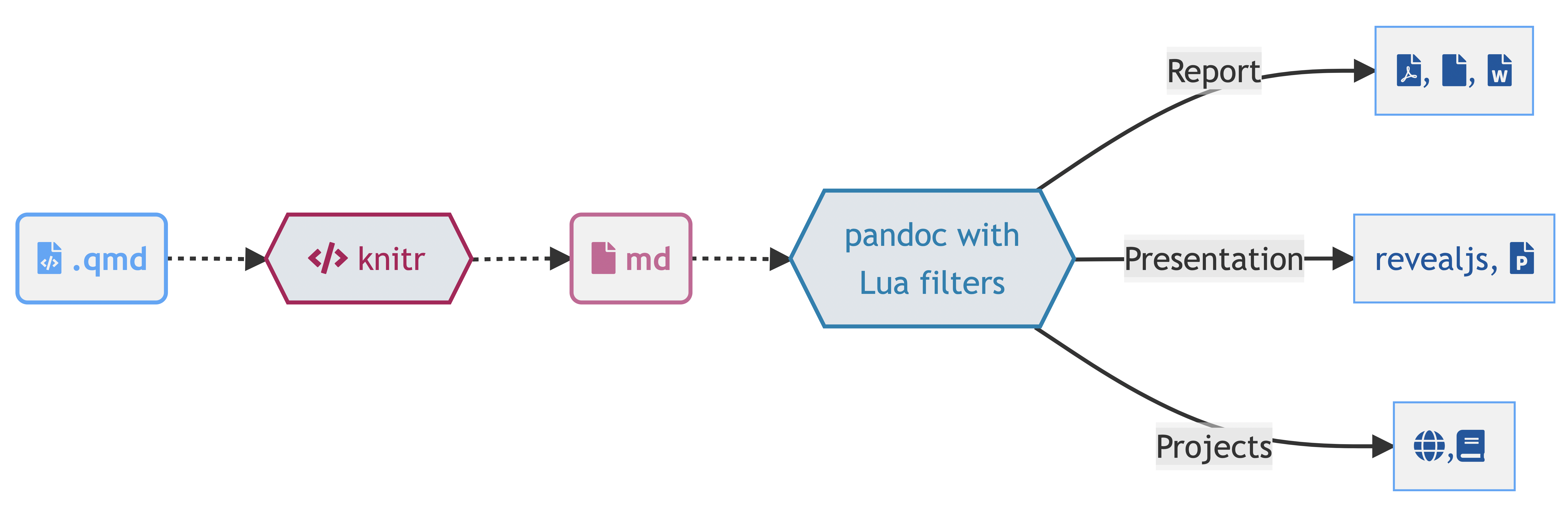
Quarto uses the {knitr} engine just like RMarkdown to execute R code natively, along with many other languages.
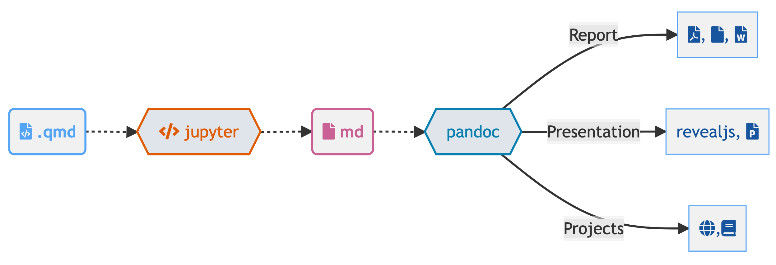
Quarto can also use the Jupyter engine to natively execute Julia, Python, or other languages that Jupyter supports.
Start your engine!
Code
Code, more than just R
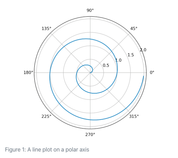
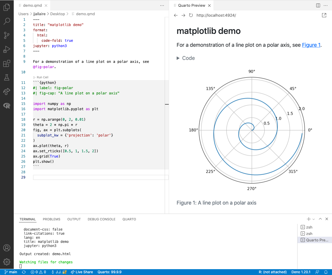
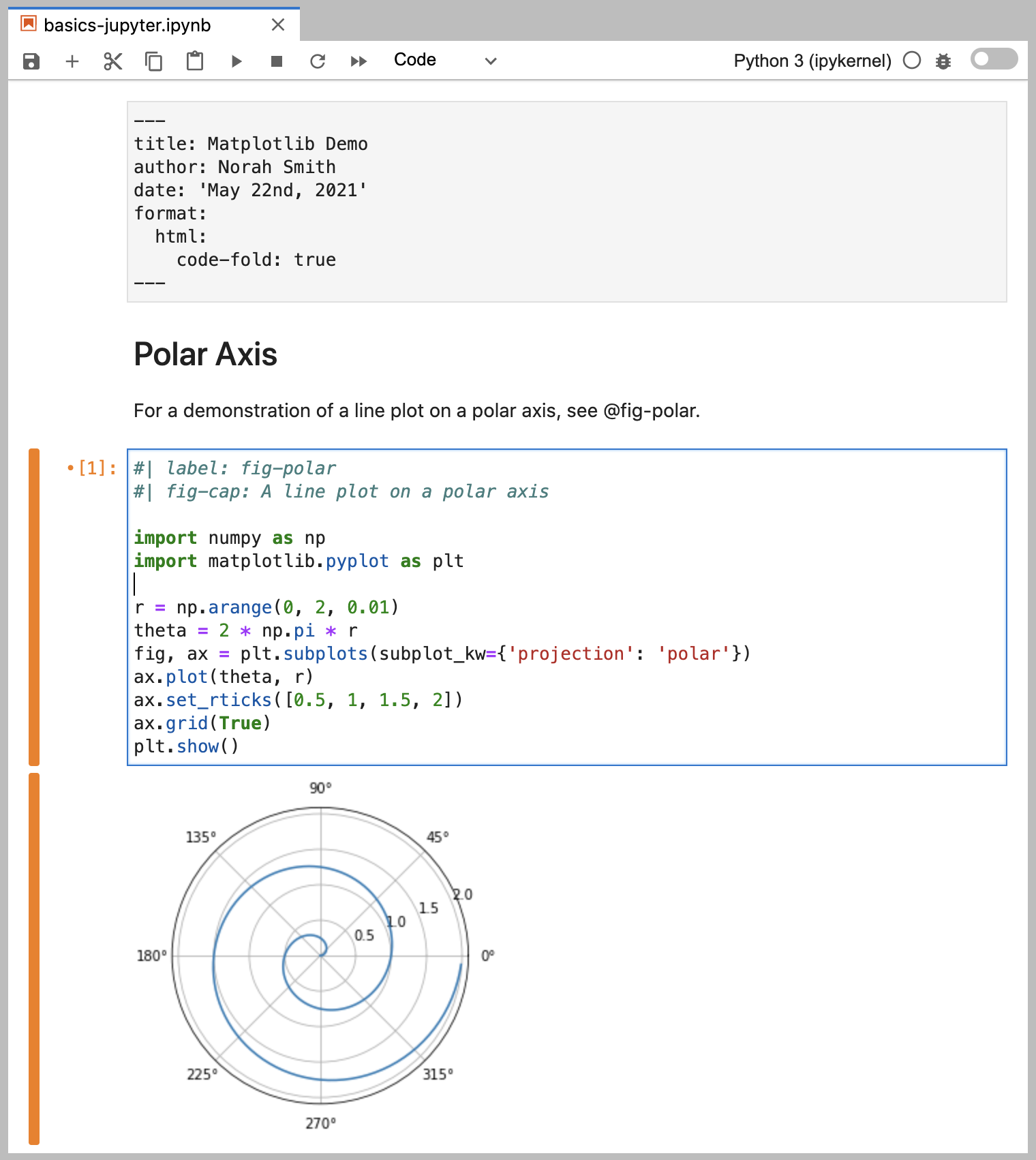
```{python}
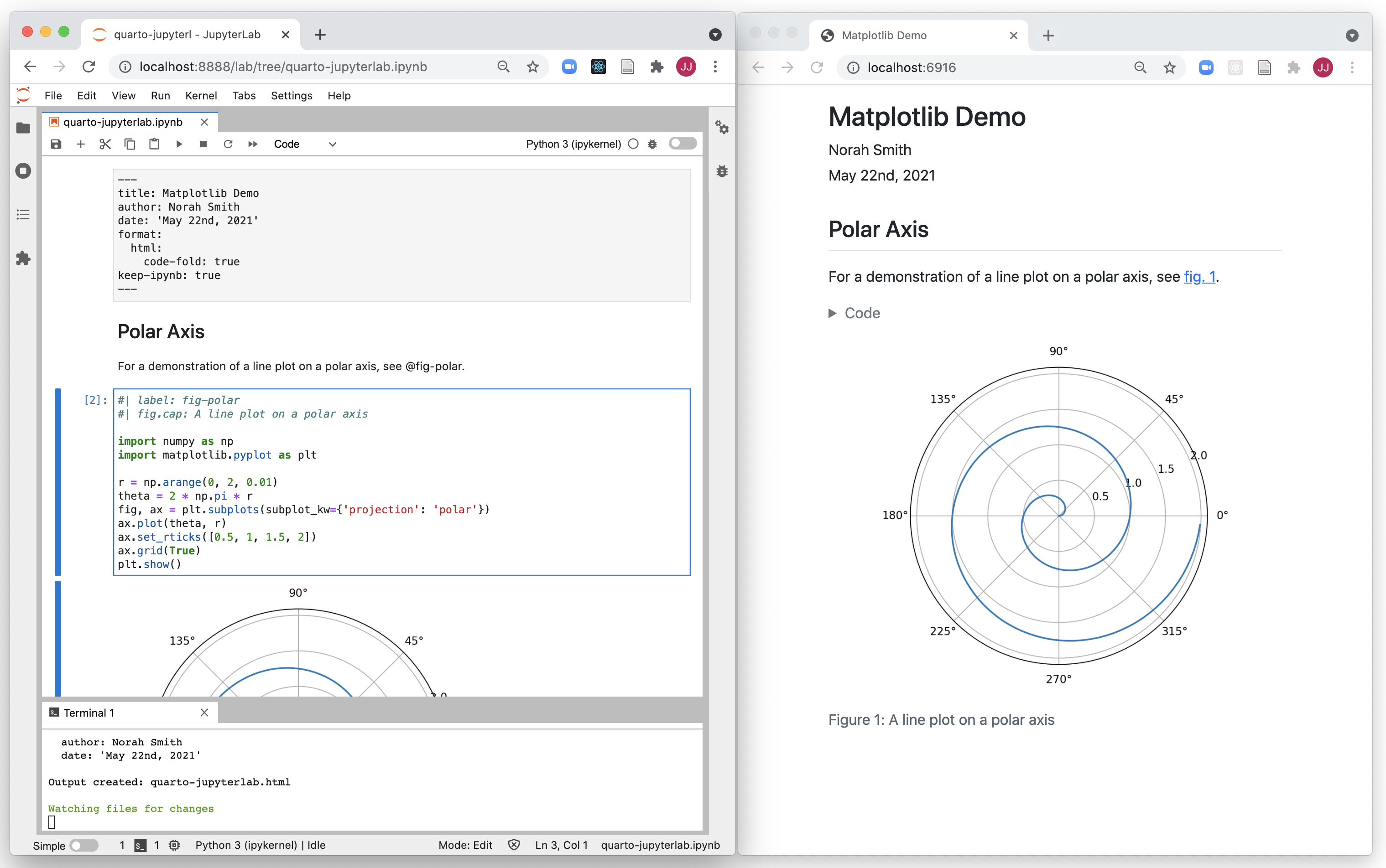
#| label: fig-polar
#| eval: false
#| fig-cap: "A line plot on a polar axis"
import numpy as np
import matplotlib.pyplot as plt
r = np.arange(0, 2, 0.01)
theta = 2 * np.pi * r
fig, ax = plt.subplots(
subplot_kw = {'projection': 'polar'}
)
ax.plot(theta, r)
ax.set_rticks([0.5, 1, 1.5, 2])
ax.grid(True)
plt.show()
```
Quarto’s hash pipe #|

Quarto chunk options
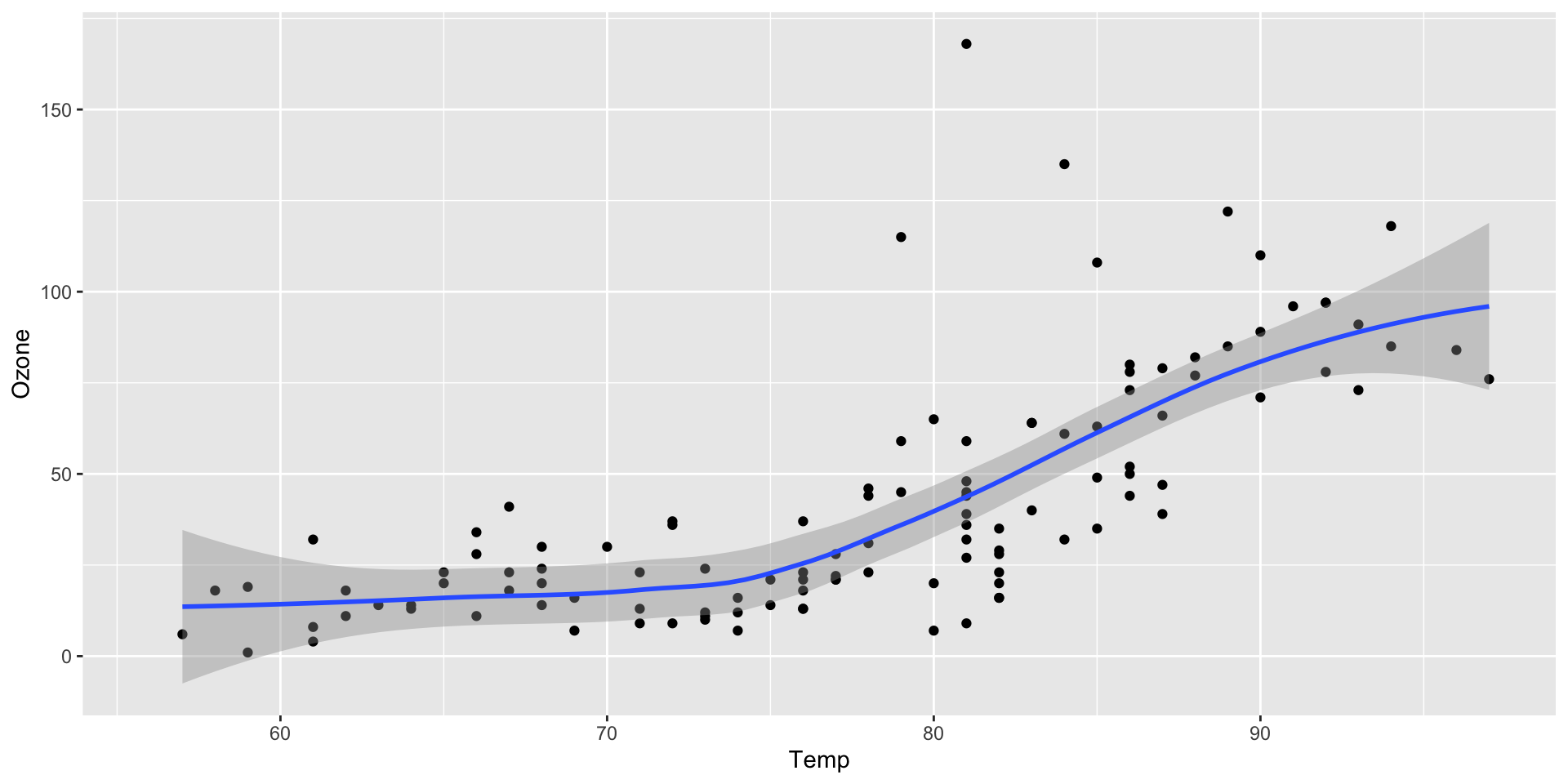
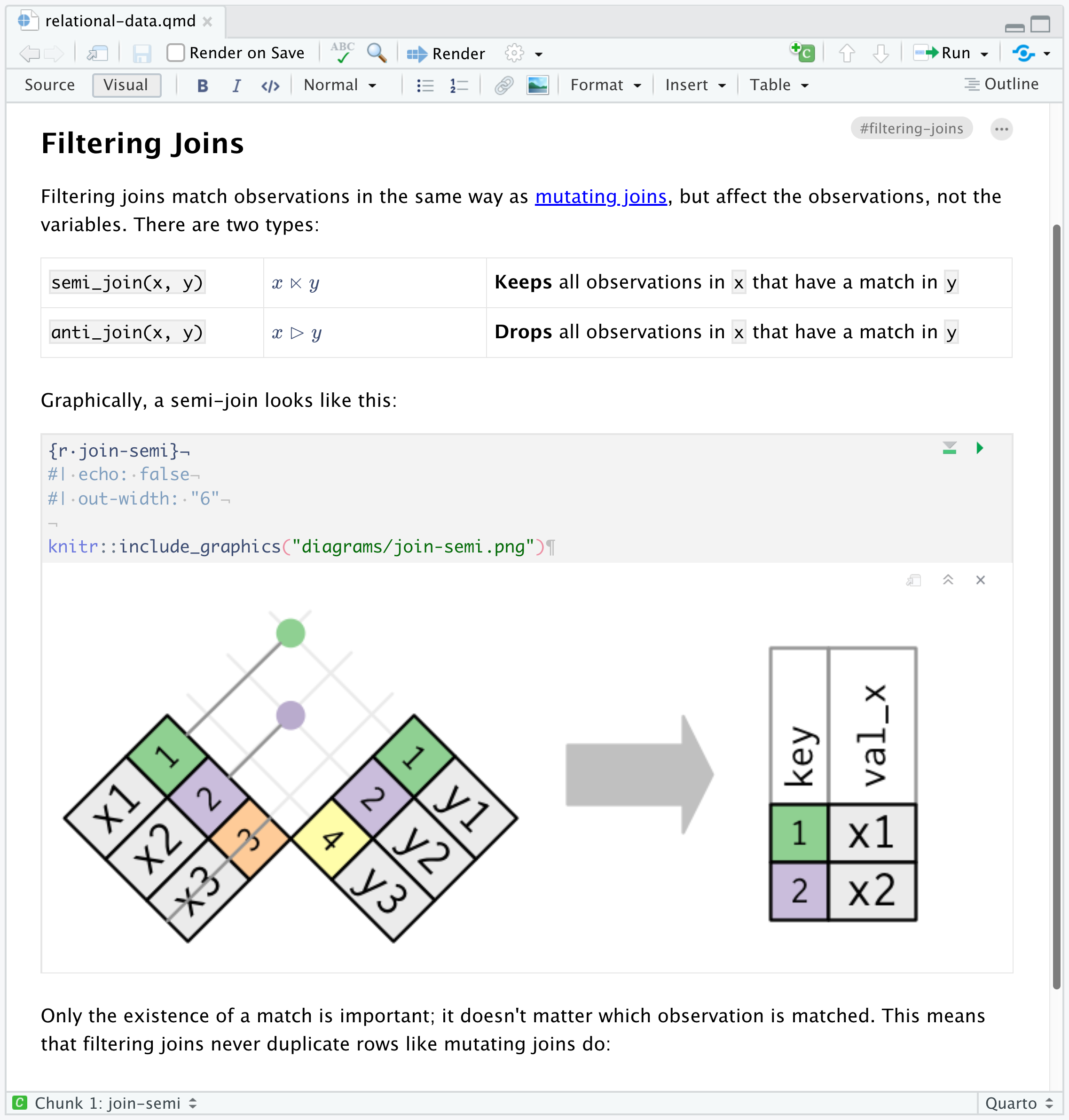
```{r}
#| warning: false
#| fig-cap: "Air Quality"
#| fig-alt: "A ggplot2 with temperature by ozone levels along with a trend line indicating the increase in temperature with increasing ozone levels."

library(ggplot2)
ggplot(airquality, aes(Ozone, Temp)) +
        geom_point() +
        geom_smooth(method = "loess", se = FALSE)
```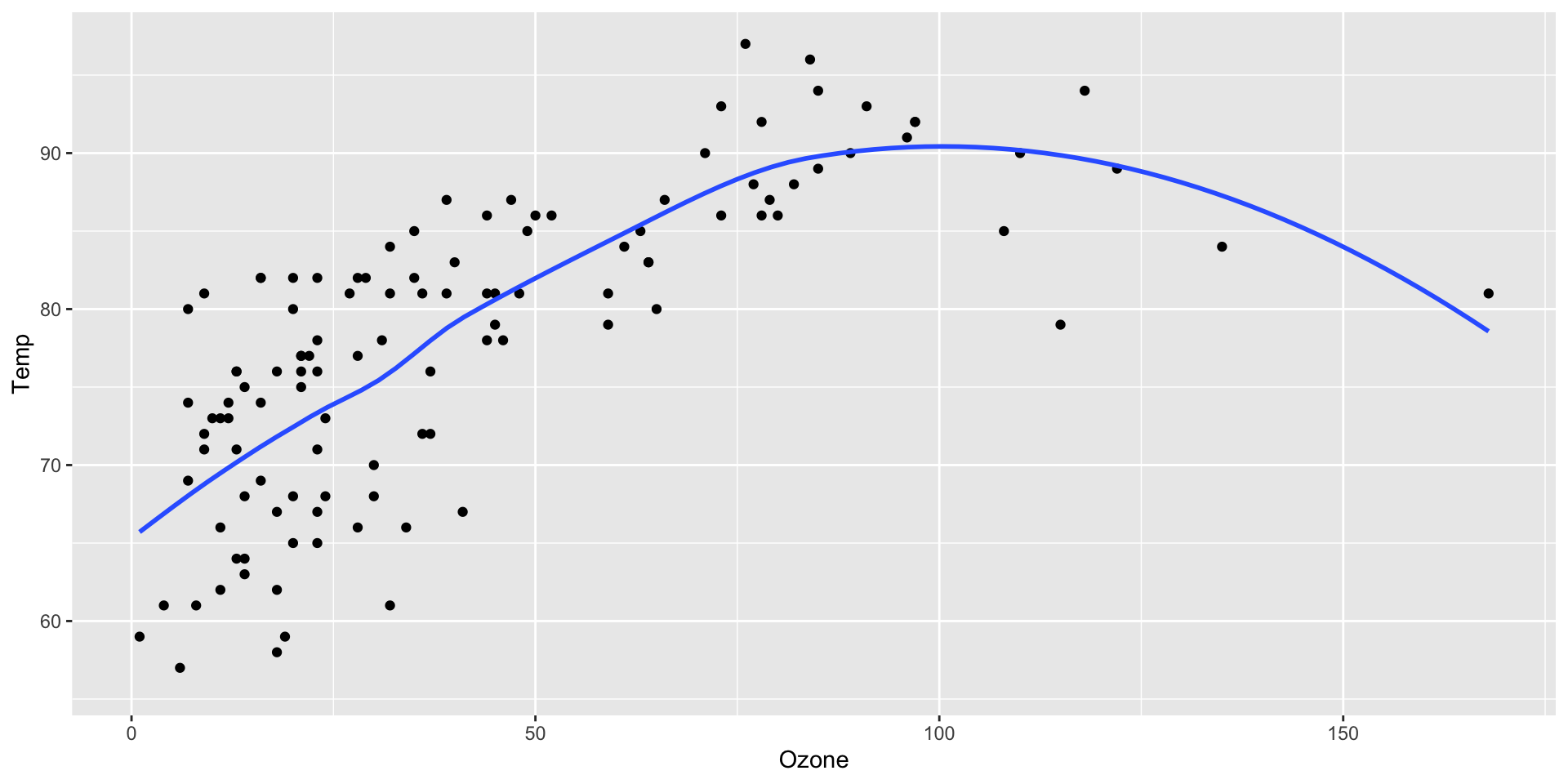
Air Quality
RMarkdown vs Quarto
You can mix and match or use only R Markdown or Quarto style knitr options. However, note the difference between ‘naming’ of the chunk options, typically one.two vs one-two. The one.two exists for backwards compatibility and you should focus on one-two syntax.
fig.align vs fig-align
fig.dpi vs fig-dpi
This syntax is preferred because it aligns with Pandoc, which uses word1-word2 style
Chunks can be named
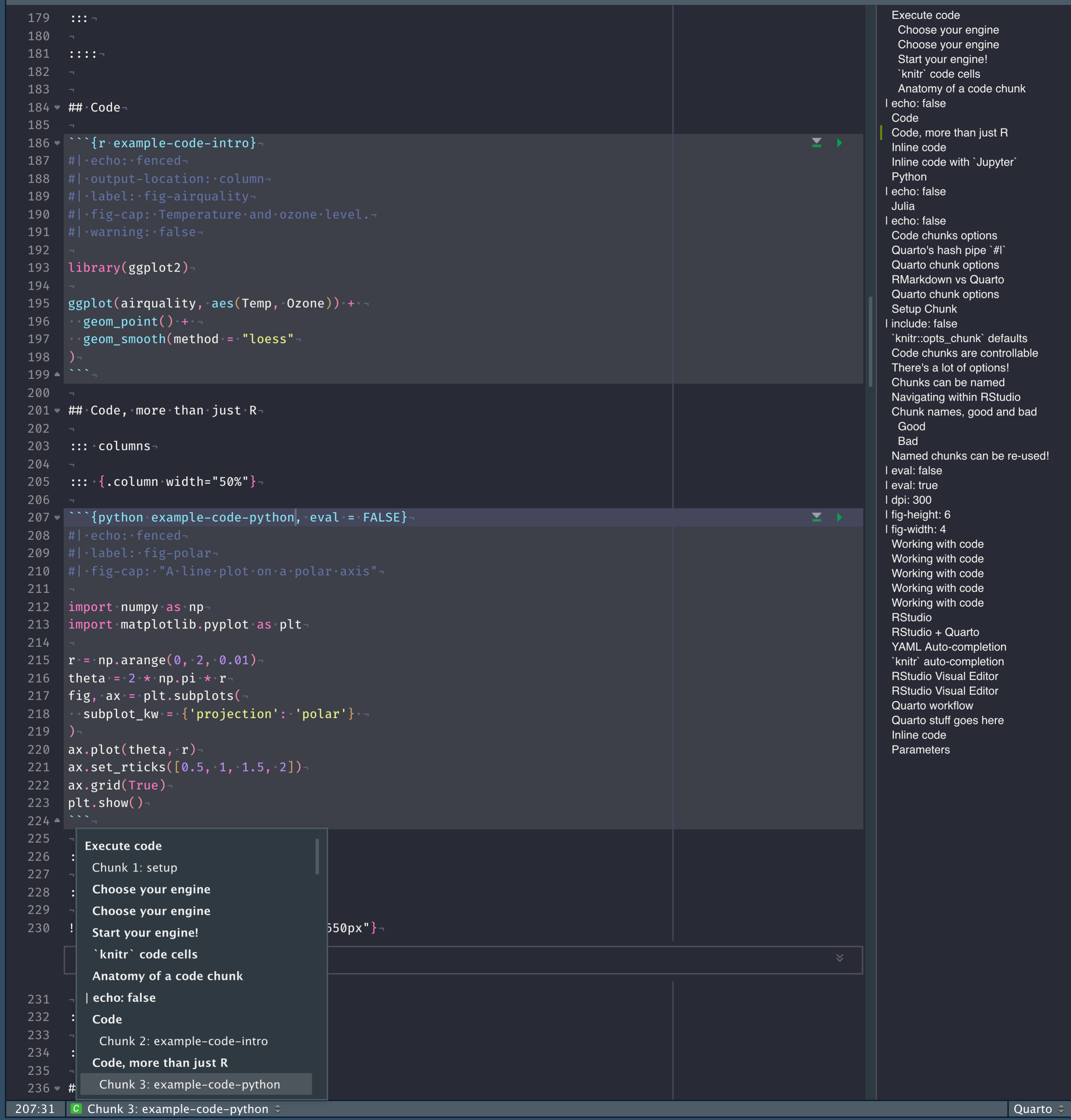
- Useful for troubleshooting (ie where is the document failing on render)
label: unnamed-chunk-23
  |..............................|  83%
  ordinary text without R code
  |..............................|  85%
label: unnamed-chunk-24 (with options)
List of 2
 $ fig.dim: num [1:2] 6 4
 $ dpi    : num 150
  |..............................|  86%
ordinary text without R codeNamed chunks can be re-used!
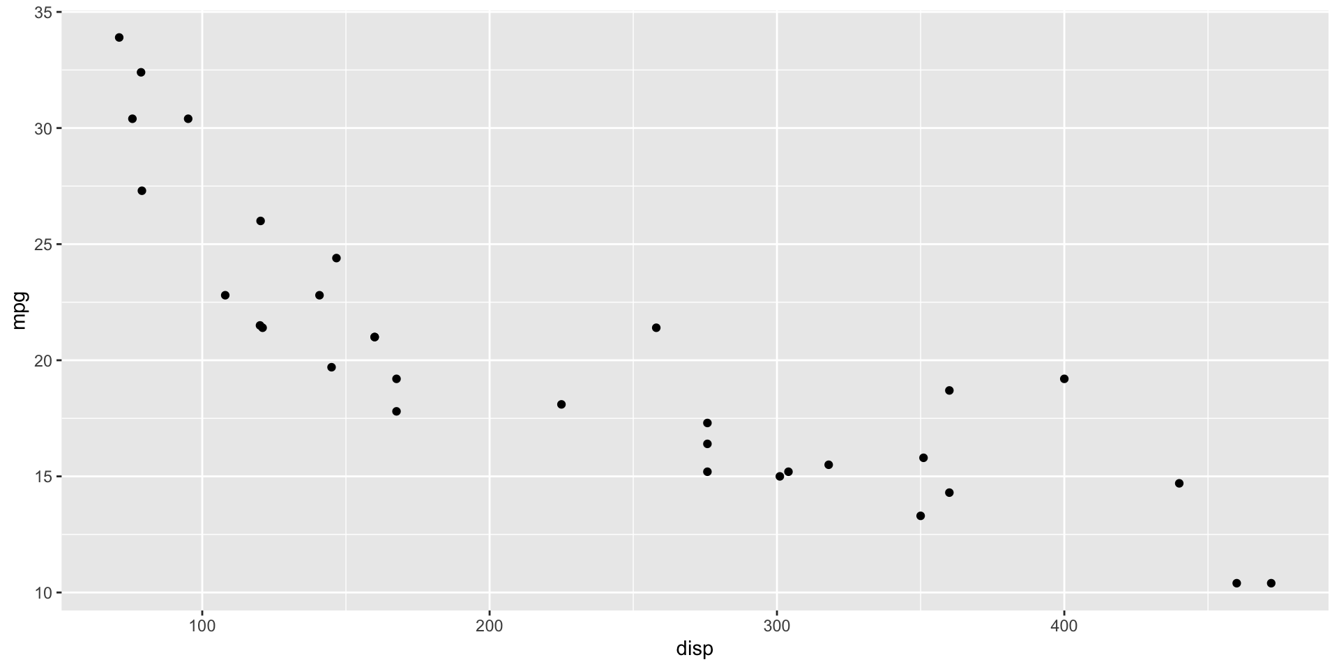
```{r}
#| label: myPlt
#| eval: false
ggplot(mtcars, aes(x = disp, y = mpg,
    color = factor(cyl))) +
  geom_point()
```
Note that you when using named chunks you can’t alter the internal code, only the chunk options. This is necessary because you are referencing the initially defined code in that chunk.

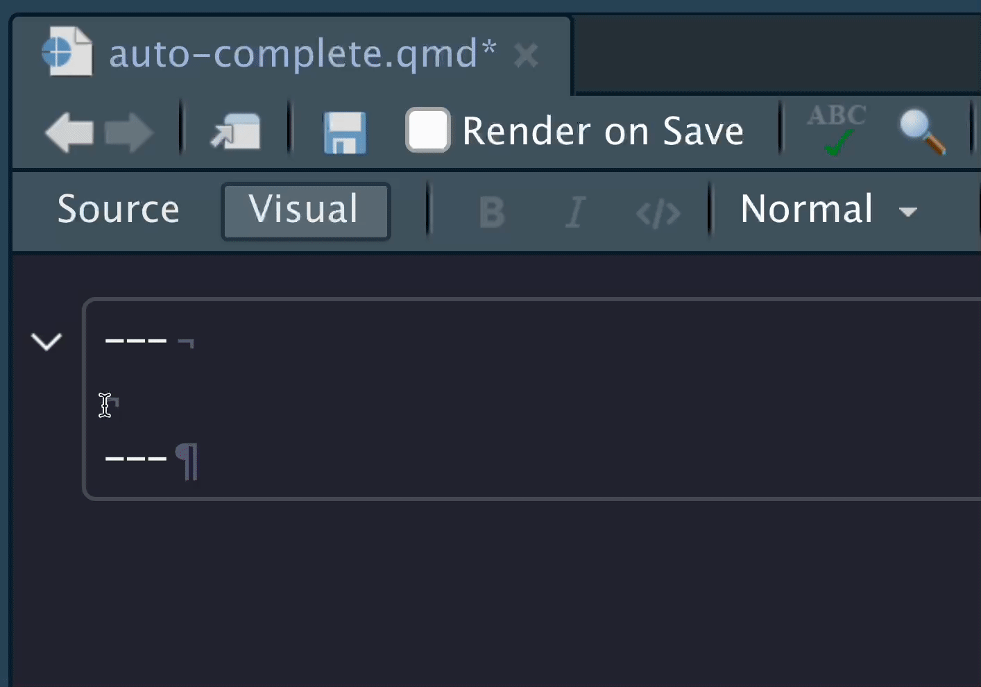
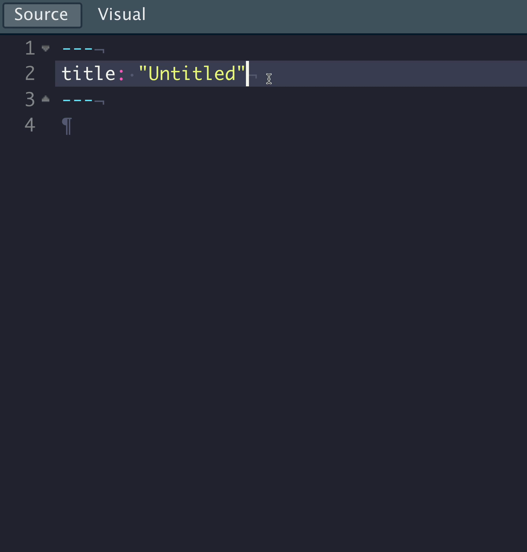
YAML Auto-completion
Quarto + RStudio provides a rich YAML auto-completion based on text.
 ## YAML Auto-completion
To find all the available options for a YAML section, you can use Ctrl + Space
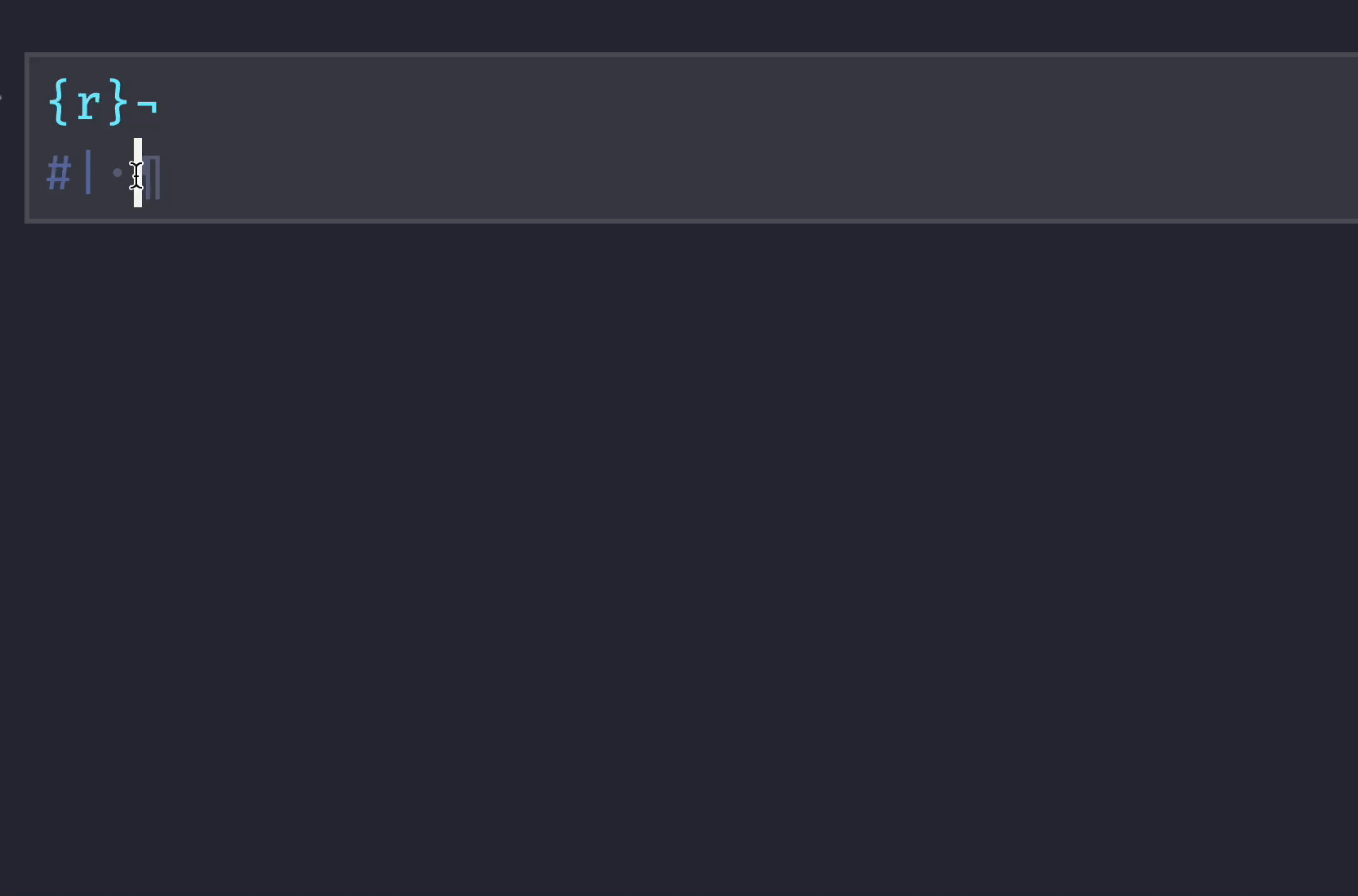
knitr auto-completion
You can use tab-completion inside knitr chunk options for RMarkdown style or Quarto style as well.
RStudio Visual Editor
VS Code
VS Code YAML
VS Code, YAML Intelligence
Jupyter/Jupyter Lab
Jupyter
quarto preview notebook.ipynb --to html
Jupyter YAML
Treat YAML as a “raw cell” in Jupyter - Jupyter doesn’t care about YAML, but it’s needed/used by Quarto
Your Turn
thomasmock$ quarto --help

  Usage:   quarto
  Version: 1.0.36

  Description:
    Quarto CLI

  Options:
    -h, --help     - Show this help.
    -V, --version  - Show the version number for this program.

  Commands:
    render          [input] [args...]   - Render input file(s) to various document types.
    preview         [file] [args...]    - Render and preview a document or website project.
    serve           [input]             - Serve a Shiny interactive document.
    create-project  [dir]               - Create a project for rendering multiple documents
    convert         <input>             - Convert documents to alternate representations.
    pandoc          [args...]           - Run the version of Pandoc embedded within Quarto.
    run             [script] [args...]  - Run a TypeScript, R, Python, or Lua script.
    install         <type> [target]     - Installs an extension or global dependency.
    publish         [provider] [path]   - Publish a document or project. Available providers include:
    check           [target]            - Verify correct functioning of Quarto installation.
    help            [command]           - Show this help or the help of a sub-command.