Getting Started with Shiny
Day 1

Colin Rundel

Introduction to Shiny

Shiny

Shiny is an R package that makes it easy to build interactive web apps straight from R. You can host standalone apps on a webpage or embed them in R Markdown documents or build dashboards. You can also extend your Shiny apps with CSS themes, htmlwidgets, and JavaScript actions.

Shiny App

Server

+

⇄

Client / Browser

+ +

Anatomy of an App

library(shiny)

shinyApp(
  ui = list(),
  
  server = function(input, output, session) {
  
  }
)

Demo 1 - A Basic Example

demos/demo1.R

library(tidyverse)
library(shiny)
d = readr::read_csv(here::here("data/weather.csv"))

shinyApp(
  ui = fluidPage(
    titlePanel("Temperature Forecasts"),
    sidebarLayout(
      sidebarPanel(
        radioButtons(
          "city", "Select a city",
          choices = c("Washington", "New York", "Los Angeles", "Chicago")
        ) 
      ),
      mainPanel( plotOutput("plot") )
    )
  ),
  server = function(input, output, session) {
    output$plot = renderPlot({
      d %>%
        filter(city %in% input$city) %>%
        ggplot(aes(x=time, y=temperature, color=city)) +
        geom_line()
    })
  }
)

Your turn - Exercise 1

Copy the code from the previous slide (or open `exercises/ex1.R) and try running it in your console.

Check that you are able successfully run the shiny app and are able to interact with it.

• If everything is working try modifying the code (e.g. try adding or removing a city from radioButtons()).

• What happens if you add a city that is not in the weather.csv data set?

Troubleshooting

A couple of quick tips:

• If you can find the data, make sure you have opened the workshop’s RStudio project

• Make sure you have the latest versions of shiny and tidyverse installed

• If you are stuck, ask a neighbor for help and or raise your hand

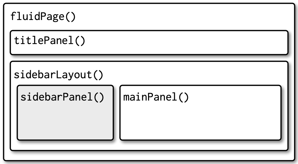
Layouts

Sidebar layout

From Mastering Shiny

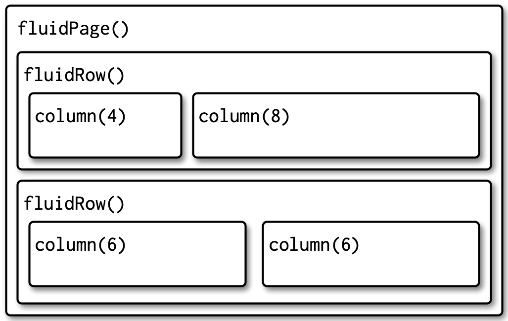
Multi-row layout

From Mastering Shiny

Other layouts

• Tabsets - see tabsetPanel()

• Navbars and navlists

  • See navlistPanel()
  • and navbarPage()

• Shinydashboard

Input Widgets

Shiny Widgets Gallery

shiny.rstudio.com/gallery/widget-gallery.html

A brief widget tour

rundel.shinyapps.io/widgets/

Take a look at widgets/widgets.qmd if you want to see how this was built.

Your turn - Exercise 2

We’ve just seen a number of alternative input widgets, starting from the code in exercises/ex2.R try changing the radioButton() input to something else.

What happens if you use an input capable of selecting multiple values

• e.g. checkboxGroupInput()
• or selectInput(multiple = TRUE)?

Basic Reactivity

Reactive elements

demos/demo1.R

library(tidyverse)
library(shiny)
d = readr::read_csv(here::here("data/weather.csv"))

shinyApp(
  ui = fluidPage(
    titlePanel("Temperature Forecasts"),
    sidebarLayout(
      sidebarPanel(
        radioButtons(
          "city", "Select a city",
          choices = c("Washington", "New York", "Los Angeles", "Chicago")
        ) 
      ),
      mainPanel( plotOutput("plot") )
    )
  ),
  server = function(input, output, session) {
    output$plot = renderPlot({
      d %>%
        filter(city %in% input$city) %>%
        ggplot(aes(x=time, y=temperature, color=city)) +
        geom_line()
    })
  }
)

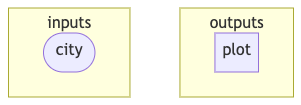
Our inputs and outputs are defined by our ui elements.

Reactive expression

demos/demo1.R

library(tidyverse)
library(shiny)
d = readr::read_csv(here::here("data/weather.csv"))

shinyApp(
  ui = fluidPage(
    titlePanel("Temperature Forecasts"),
    sidebarLayout(
      sidebarPanel(
        radioButtons(
          "city", "Select a city",
          choices = c("Washington", "New York", "Los Angeles", "Chicago")
        ) 
      ),
      mainPanel( plotOutput("plot") )
    )
  ),
  server = function(input, output, session) {
    output$plot = renderPlot({
      d %>%
        filter(city %in% input$city) %>%
        ggplot(aes(x=time, y=temperature, color=city)) +
        geom_line()
    })
  }
)

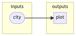
The “reactive” logic is defined by our server function - shiny takes care of figuring out what depends on what.

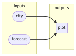
Demo 2 - Adding an input

demos/demo2.R

library(tidyverse)
library(shiny)
d = readr::read_csv(here::here("data/weather.csv"))

shinyApp(
  ui = fluidPage(
    titlePanel("Temperature Forecasts"),
    sidebarLayout(
      sidebarPanel(
        radioButtons(
          "city", "Select a city",
          choices = c("Washington", "New York", "Los Angeles", "Chicago")
        ),
        checkboxInput("forecast", "Highlight forecasted data", value = FALSE)
      ),
      mainPanel( plotOutput("plot") )
    )
  ),
  server = function(input, output, session) {
    output$plot = renderPlot({
      g = d %>%
        filter(city %in% input$city) %>%
        ggplot(aes(x=time, y=temperature, color=city)) +
        geom_line()
      
      if (input$forecast) {
        g = g + geom_rect(inherit.aes = FALSE,
          data = d %>%
            filter(forecast) %>%
            group_by(forecast) %>%
            summarize(xmin = min(time)),
          aes(xmin=xmin),
          ymin = -Inf, ymax = Inf, xmax=Inf,
          alpha = 0.25, color = NA, fill = "yellow"
        )
      }
      
      g
    })
  }
)

Reactive graph

With these additions, what should our reactive graph look like now?

Reactive graph

With these additions, what should our reactive graph look like now?

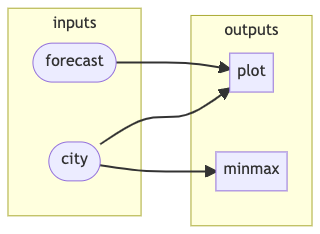
Your turn - Exercise 3

Starting with the demo 2 code in exercises/ex3.R add a tableOutput() to the app’s mainPanel().

Once you have done that you should then add logic to the server function to render a table that shows the daily min and max temperature for each day of the week.

• You will need to use renderTable()
• lubridate::wday() is likely to be useful along with group_by() & summarize()

Reactive graph (again)

reactlog

Another (more detailed) way of seeing the reactive graph (dynamically) for your app is using the reactlog package.

Run the following to log and show all of the reactive events occuring within ex3_soln.R,

reactlog::reactlog_enable()

(source(here::here("exercises/solutions/ex3_soln.R")))

shiny::reactlogShow()

User selected variables

Demo 3 - Not just temperature

demos/demo3.R

library(tidyverse)
library(shiny)
d = readr::read_csv(here::here("data/weather.csv"))

d_vars = d %>%
  select(where(is.numeric)) %>%
  names()

shinyApp(
  ui = fluidPage(
    titlePanel("Weather Forecasts"),
    sidebarLayout(
      sidebarPanel(
        radioButtons(
          "city", "Select a city",
          choices = c("Washington", "New York", "Los Angeles", "Chicago")
        ),
        selectInput(
          "var", "Select a variable",
          choices = d_vars, selected = "temperature"
        )
      ),
      mainPanel( 
        plotOutput("plot"),
        tableOutput("minmax")
      )
    )
  ),
  server = function(input, output, session) {
    output$plot = renderPlot({
      d %>%
        filter(city %in% input$city) %>%
        ggplot(aes(x=time, y=.data[[input$var]], color=city)) +
        ggtitle(input$var) +
        geom_line()
    })
    
    output$minmax = renderTable({
      d %>%
        filter(city %in% input$city) %>%
        mutate(
          day = lubridate::wday(time, label = TRUE, abbr = FALSE),
          date = as.character(lubridate::date(time))
        ) %>%
        group_by(date, day) %>%
        summarize(
          `min` = min(.data[[input$var]]),
          `max` = max(.data[[input$var]]),
          .groups = "drop"
        )
    })
  }
)

.data & .env

These are an excellent option for avoiding some of the complexity around NSE with rlang (e.g. {{, !!, enquo(), etc.) when working with functions built with the tidy eval framework (e.g. dplyr and ggplot2).

• .data retrieves data-variables from the data frame.
• .env retrieves env-variables from the environment.

For more details see the rlang .data and .env pronouns article.

reactive() & observe()

Don’t repeat yourself (DRY)

demos/demo3.R

library(tidyverse)
library(shiny)
d = readr::read_csv(here::here("data/weather.csv"))

d_vars = d %>%
  select(where(is.numeric)) %>%
  names()

shinyApp(
  ui = fluidPage(
    titlePanel("Weather Forecasts"),
    sidebarLayout(
      sidebarPanel(
        radioButtons(
          "city", "Select a city",
          choices = c("Washington", "New York", "Los Angeles", "Chicago")
        ),
        selectInput(
          "var", "Select a variable",
          choices = d_vars, selected = "temperature"
        )
      ),
      mainPanel( 
        plotOutput("plot"),
        tableOutput("minmax")
      )
    )
  ),
  server = function(input, output, session) {
    output$plot = renderPlot({
      d %>%
        filter(city %in% input$city) %>%
        ggplot(aes(x=time, y=.data[[input$var]], color=city)) +
        ggtitle(input$var) +
        geom_line()
    })
    
    output$minmax = renderTable({
      d %>%
        filter(city %in% input$city) %>%
        mutate(
          day = lubridate::wday(time, label = TRUE, abbr = FALSE),
          date = as.character(lubridate::date(time))
        ) %>%
        group_by(date, day) %>%
        summarize(
          `min` = min(.data[[input$var]]),
          `max` = max(.data[[input$var]]),
          .groups = "drop"
        )
    })
  }
)

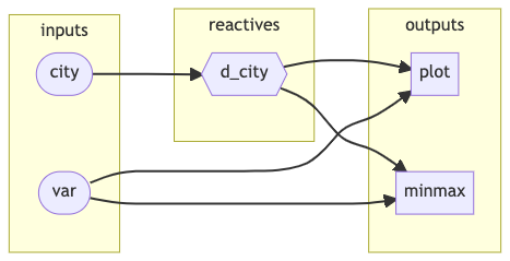
Demo 4 - Use a reactive

demos/demo4.R

library(tidyverse)
library(shiny)
d = readr::read_csv(here::here("data/weather.csv"))

d_vars = d %>%
  select(where(is.numeric)) %>%
  names()

shinyApp(
  ui = fluidPage(
    titlePanel("Weather Forecasts"),
    sidebarLayout(
      sidebarPanel(
        radioButtons(
          "city", "Select a city",
          choices = c("Washington", "New York", "Los Angeles", "Chicago")
        ),
        selectInput(
          "var", "Select a variable",
          choices = d_vars, selected = "temperature"
        )
      ),
      mainPanel( 
        plotOutput("plot"),
        tableOutput("minmax")
      )
    )
  ),
  server = function(input, output, session) {
    
    d_city = reactive({
      d %>%
        filter(city %in% input$city)
    })
    
    output$plot = renderPlot({
      d_city() %>%
        ggplot(aes(x=time, y=.data[[input$var]], color=city)) +
        ggtitle(input$var) +
        geom_line()
    })
    
    output$minmax = renderTable({
      d_city() %>%
        mutate(
          day = lubridate::wday(time, label = TRUE, abbr = FALSE),
          date = as.character(lubridate::date(time))
        ) %>%
        group_by(date, day) %>%
        summarize(
          `min` = min(.data[[input$var]]),
          `max` = max(.data[[input$var]]),
          .groups = "drop"
        )
    })
  }
)

Reactive expressions

Are an example of a “reactive conductor” as they exist in between sources (e.g. an input) and endpoints (e.g. an output).

As such a reactive() depends on various upstream inputs and can be used to generate output.

Their primary use is similar to a function in an R script, they help to

• avoid repeating yourself

• decompose complex computations into smaller / more modular steps

• can improve computational efficiency by breaking up / simplifying reactive dependencies

reactive() tips

• Code written similarly to render*() functions

• If react_obj = reactive({...}) then any consumer must access value using react_obj() and not react_obj

  • think of react_obj as a function that returns the current value

  • Common cause of everyone’s my favorite R error ,

    ## Error: object of type 'closure' is not subsettable`

• Like inputs reactive expressions may only be used within a reactive context (e.g. render*(), reactive(), observer(), etc.)

  ## Error: Operation not allowed without an active reactive context. (You tried to do something that can only be done from inside a reactive expression or observer.)

Reactive graph

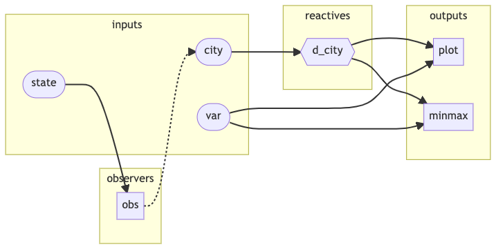
observer()

These are constructed in the same way as a reactive() however an observer does not return a value, as such they are used for their side effects.

• The side effects in most cases involve sending data to the client broswer, e.g. updating a UI element

• While not obvious given their syntax - the results of the render*() functions are observers.

Demo 5 - Cities AND states

demos/demo5.R

library(tidyverse)
library(shiny)
d = readr::read_csv(here::here("data/weather.csv"))

d_vars = d %>%
  select(where(is.numeric)) %>%
  names()

shinyApp(
  ui = fluidPage(
    titlePanel("Weather Forecasts"),
    sidebarLayout(
      sidebarPanel(
        selectInput(
          "state", "Select a state",
          choices = sort(unique(d$state))
        ),
        selectInput(
          "city", "Select a city",
          choices = c(),
          multiple = TRUE
        ),
        selectInput(
          "var", "Select a variable",
          choices = d_vars, selected = "temperature"
        )
      ),
      mainPanel( 
        plotOutput("plot"),
        tableOutput("minmax")
      )
    )
  ),
  server = function(input, output, session) {
    
    d_city = reactive({
      req(input$city)
      d %>%
        filter(city %in% input$city)
    })
    
    observe({
      cities = d %>%
        filter(state %in% input$state) %>%
        pull(city) %>%
        unique() %>%
        sort()
      
      updateSelectInput(
        inputId = "city", 
        choices = cities
      )
    })
    
    output$plot = renderPlot({
      d_city() %>%
        ggplot(aes(x=time, y=.data[[input$var]], color=city)) +
        ggtitle(input$var) +
        geom_line()
    })
    
    output$minmax = renderTable({
      d_city() %>%
        mutate(
          day = lubridate::wday(time, label = TRUE, abbr = FALSE),
          date = as.character(lubridate::date(time))
        ) %>%
        group_by(date, day) %>%
        summarize(
          `min` = min(.data[[input$var]]),
          `max` = max(.data[[input$var]]),
          .groups = "drop"
        )
    })
  }
)

Reactive graph

Using req()

You may have notices that the App initializes with Arizona selected for the state but no initial selection for the city. Due to this we have some warnings generated initially:

Warning in min(.data[["temperature"]]) :
  no non-missing arguments to min; returning Inf

This can be a common occurrence, particularly at initialization (or if a user enters bad / unexpected input).

A good way to protect against this is to validate inputs - the simplest way is to use req() which checks if a value is truthy. Non-truthy values prevent further execution of the reactive code (and downstream consumer’s code).

More detailed validation and error reporting is possible with validate() and need().

A cautionary example

library(shiny)

shinyApp(
  ui <- fluidPage(
    numericInput("n", "n", 0)
  ),
  server <- function(input, output, session) {
    observeEvent(input$n,
      updateNumericInput(inputId = "n", value = input$n + 1)
    )
  }
)

From Mastering Shiny

Your turn - Exercise 4

Using the code from demo 4 as a starting point add another observer to the app that updates the selectInput() for var such that any variables that are constant (0 variance), for the currently selected cities, are removed.

For example, many cities (e.g. Mesa, AZ) will report a visibility of 10 miles for every hour of the forecast - therefore this variable should not be selectable from the var input.

Hint - think about what inputs / reactives would make the most sense to use for this.

bindEvent()

For both observers and reactive expressions Shiny will automatically determine reactive dependencies for you - in some cases this is not what we want.

To explicitly control the reactive dependencies of reactive expressions, render functions, and observers we can modify them using bindEvent() where the dependencies are explicitly provided via the ... argument.

Similar effects can be achieved via observeEvent() / eventReactive() but these have been soft deprecated as of Shiny 1.6.

Note - when binding a reactive you must use the functional form, i.e. react() and not react

Downloading from Shiny

downloadButton() & downloadHandler()

These are the UI and server components needed for downloading a file from your Shiny app. The downloaded file can be of any arbitrary type and content.

downloadButton() is a special case of an actionButton() with specialized server syntax.

Specifically, within the server definition the downloadHandler() is attached to the button’s id via output, e.g.

output$download_btn = downloadHandler(...)

The handler then defines the filename function for generating a default filename and content function for writing the download file’s content to a temporary file, which can then be served by Shiny for downloading.

Demo 6 - A download button

demos/demo6.R

library(tidyverse)
library(shiny)
d = readr::read_csv(here::here("data/weather.csv"))

d_vars = d %>%
  select(where(is.numeric)) %>%
  names()

shinyApp(
  ui = fluidPage(
    titlePanel("Weather Forecasts"),
    sidebarLayout(
      sidebarPanel(
        selectInput(
          "state", "Select a state",
          choices = sort(unique(d$state))
        ),
        selectInput(
          "city", "Select a city",
          choices = c(),
          multiple = TRUE
        ),
        selectInput(
          "var", "Select a variable",
          choices = d_vars, selected = "temperature"
        ),
        downloadButton("download")
      ),
      mainPanel( 
        plotOutput("plot"),
        tableOutput("minmax")
      )
    )
  ),
  server = function(input, output, session) {
    
    output$download = downloadHandler(
      filename = function() {
        paste0(
          paste(input$city,collapse="_"), 
          ".csv"
        )
      },
      content = function(file) {
        readr::write_csv(d_city(), file)
      }
    )
    
    d_city = reactive({
      req(input$city)
      d %>%
        filter(city %in% input$city)
    })
    
    observe({
      cities = d %>%
        filter(state %in% input$state) %>%
        pull(city) %>%
        unique() %>%
        sort()
      
      updateSelectInput(
        inputId = "city", 
        choices = cities
      )
    })
    
    output$plot = renderPlot({
      d_city() %>%
        ggplot(aes(x=time, y=.data[[input$var]], color=city)) +
        ggtitle(input$var) +
        geom_line()
    })
    
    output$minmax = renderTable({
      d_city() %>%
        mutate(
          day = lubridate::wday(time, label = TRUE, abbr = FALSE),
          date = as.character(lubridate::date(time))
        ) %>%
        group_by(date, day) %>%
        summarize(
          `min` = min(.data[[input$var]]),
          `max` = max(.data[[input$var]]),
          .groups = "drop"
        )
    })
  }
)

Modal dialogs

These are a popup window element that allow us to present important messages (e.g. warnings or errors) or other UI elements in a way that does not permanently clutter up the main UI of an app.

The modal dialog consists of a number of Shiny UI elements (static or dynamic) and only displays when it is triggered (usually by something like an action button or link).

They differ from other UI elements we’ve seen so far as they are usually defined within an app’s server component not the ui.

Demo 7 - A fancy download button

demos/demo7.R

library(tidyverse)
library(shiny)
d = readr::read_csv(here::here("data/weather.csv"))
d_vars = d %>%
  select(where(is.numeric)) %>%
  names()

shinyApp(
  ui = fluidPage(
    titlePanel("Weather Forecasts"),
    sidebarLayout(
      sidebarPanel(
        selectInput(
          "state", "Select a state",
          choices = sort(unique(d$state))
        ),
        selectInput(
          "city", "Select a city",
          choices = c(),
          multiple = TRUE
        ),
        selectInput(
          "var", "Select a variable",
          choices = d_vars, selected = "temperature"
        ),
        actionButton("download_modal", "Download")
      ),
      mainPanel( 
        plotOutput("plot"),
        tableOutput("minmax")
      )
    )
  ),
  server = function(input, output, session) {
    
    observe({
      showModal(modalDialog(
        title = "Download data",
        checkboxGroupInput(
          "dl_vars", "Select variables to download",
          choices = names(d), selected = names(d), inline = TRUE
        ),
        footer = list(
          downloadButton("download"),
          modalButton("Cancel")
        )
      ))
    }) %>%
      bindEvent(input$download_modal)
    
    output$download = downloadHandler(
      filename = function() {
        paste0(
          paste(input$city,collapse="_"), 
          ".csv"
        )
      },
      content = function(file) {
        readr::write_csv(
          d_city() %>%
            select(input$dl_vars), 
          file
        )
      }
    )
    
    d_city = reactive({
      req(input$city)
      d %>%
        filter(city %in% input$city)
    })
    
    observe({
      cities = d %>%
        filter(state %in% input$state) %>%
        pull(city) %>%
        unique() %>%
        sort()
      
      updateSelectInput(
        inputId = "city", 
        choices = cities
      )
    })
    
    output$plot = renderPlot({
      d_city() %>%
        ggplot(aes(x=time, y=.data[[input$var]], color=city)) +
        ggtitle(input$var) +
        geom_line()
    })
    
    output$minmax = renderTable({
      d_city() %>%
        mutate(
          day = lubridate::wday(time, label = TRUE, abbr = FALSE),
          date = as.character(lubridate::date(time))
        ) %>%
        group_by(date, day) %>%
        summarize(
          `min` = min(.data[[input$var]]),
          `max` = max(.data[[input$var]]),
          .groups = "drop"
        )
    })
  }
)

Uploading data

Demo 8 - Using fileInput()

demos/demo8.R

library(tidyverse)
library(shiny)

shinyApp(
  ui = fluidPage(
    titlePanel("Temperature Forecasts"),
    sidebarLayout(
      sidebarPanel(
        fileInput("upload", "Upload a file")
      ),
      mainPanel( 
        tableOutput("widget"),
        tableOutput("data")
      )
    )
  ),
  server = function(input, output, session) {
    output$widget = renderTable({
      input$upload
    })
    
    output$data = renderTable({
      readr::read_csv(input$upload$datapath)
    })
  }
)

fileInput() widget

This widget behaves a bit differently than the others we have seen - once a file is uploaded it returns a data frame with one row per file and the columns,

• name - the original filename (from the client’s system)

• size - file size in bytes

• type - file mime type, usually determined by the file extension

• datapath - location of the temporary file on the server

Given this data frame your app’s server code is responsible for the actual process of reading in the uploaded file.

fileInput() hints

• input$upload will default to NULL when the app is loaded, using req(input$upload) for downstream consumers is a good idea

• Files in datapath are temporary and should be treated as ephemeral

  • additional uploads can result in the previous files being deleted

• type is at best a guess - validate uploaded files and write defensive code

• The accept argument helps to limit file types but cannot prevent bad uploads

Your turn - Exercise 5

Starting with the app version from Demo 5 (code available in exercises/ex5.R) replace the preloading of the weather data (d and d_vars) with reactive versions that are populated via a fileInput() widget.

You should then be able to get the same app behavior as before once data/weather.csv is uploaded. You can also check that your app works with the data/sedona.csv and data/gayload.csv datasets as well.

Hint - remember that anywhere that uses either d or d_vars will now need to use d() and d_vars() instead.