Getting Started with Shiny
Day 2

Colin Rundel

shinydashboard

Is a package that enables the easy generation of bootstrap based dynamic Shiny dashboards.

The core of the package is a common dashboard layout and a number of specialized UI elements (static and reactive) for creating an attractive interface.

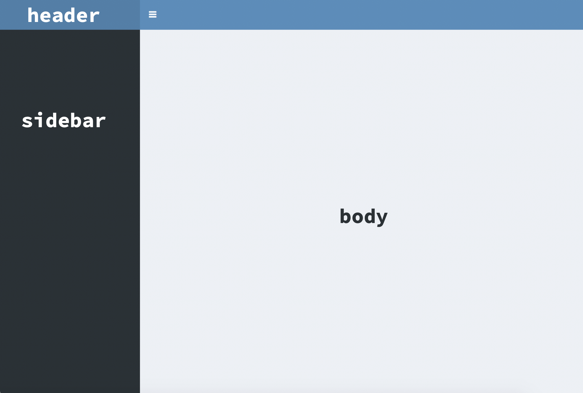
Dashboard basics

library(shiny)
library(shinydashboard)

shinyApp(
  ui = dashboardPage(
    dashboardHeader(
      title="Test"
    ),
    dashboardSidebar(),
    dashboardBody()
  ),
  server = function(input, output, session) {
  }
)

Dashboard header

This is a container for the title and any dropdownMenu()s.

Dynamic menus can be generated using:

Adding dropdownMenuOutput("menu") to the header
Adding output$menu = renderMenu({...}) to the server, where the reactive code returns a dropdownMenu() object.

This is a common design pattern within the package, so many of the static UI elements will also have a *Output() and render*() implementation.

Dashboard sidebar

This can function in the same way as the sidebarPanel() in sidebarLayout(), allowing for the inclusion of inputs and any other html content. Alternatively, it can also function as a tabPanel() like menu.

For the latter, instead of tabsetPanel() we use sidebarMenu(), text and icons are assigned using menuItem()s within this function. However, since the panels being activated are contained in the body and not the sidebar - their UI code goes under dashboardBody() using tabItems() and tabItem(). The connection is made via matching of the tabName arguments.

Body building blocks

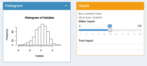
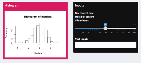
`box()`

`infoBox()`

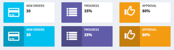
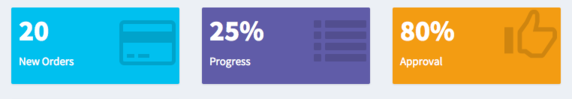
`valueBox()`

Colors

The color of the various boxes is specified via status or background for box() or color for the others.

Available options include,

shinydashboard:::validStatuses

[1] "primary" "success" "info"    "warning" "danger"

shinydashboard:::validColors

 [1] "red"        "yellow"     "aqua"       "blue"       "light-blue"
 [6] "green"      "navy"       "teal"       "olive"      "lime"      
[11] "orange"     "fuchsia"    "purple"     "maroon"     "black"

Body layout

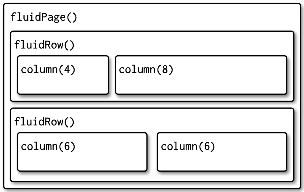
Note - Bootstrap defines a page to have a width of 12 units, a column()’s width is given in these units.

Your turn - Exercise 6

Starting with the app from Demo 5 (code available in exercises/ex6.R) convert the app to use shinydashboard instead of fluidPage() and sidebarLayout().

The specifics of the design are up to you, but think about where it makes the most sense to include the various UI elements.

See the documentation of box() and the other building blocks for guidance on how to use them, the examples here may also be useful.

If you finish early try adding a valueBox() or infoBox() (static is fine for now).

Demo 9 - Dynamic boxes

demos/demo9.R

library(tidyverse)
library(shiny)
library(shinydashboard)

d = readr::read_csv(here::here("data/weather.csv"))

d_vars = d %>%
  select(where(is.numeric)) %>%
  names()

shinyApp(
  ui = dashboardPage(
    dashboardHeader(
      title ="Weather Forecasts"
    ),
    dashboardSidebar(
      selectInput(
        "state", "Select a state",
        choices = sort(unique(d$state))
      ),
      selectInput(
        "city", "Select a city",
        choices = c(),
        multiple = TRUE
      )
      
    ),
    dashboardBody( 
      fluidRow(
        box(
          title = "Forecast", width = 12,
          solidHeader = TRUE, status = "primary",
          selectInput(
            "var", "Select a variable",
            choices = d_vars, selected = "temperature"
          ),
          plotOutput("plot")
        )
      ),
      fluidRow(
        infoBoxOutput("min_temp"),
        infoBoxOutput("max_temp"),
        infoBoxOutput("avg_wind")
      )
    )
  ),
  server = function(input, output, session) {
    
    output$min_temp = renderInfoBox({
      min_temp = min(d_city()$temperature)
      min_temp_time = d_city()$time[d_city()$temperature == min_temp]
      
      infoBox(
        title = "Min temp",
        value = min_temp,
        subtitle = format(min_temp_time, format="%a, %b %d\n%I:%M %p"),
        color = "blue",
        icon = icon("temperature-low")
      )
    })
    
    output$max_temp = renderInfoBox({
      max_temp = max(d_city()$temperature)
      max_temp_time = d_city()$time[d_city()$temperature == max_temp]
      
      infoBox(
        title = "Max temp",
        value = max_temp,
        subtitle = format(max_temp_time, format="%a, %b %d\n%I:%M %p"),
        color = "red",
        icon = icon("temperature-high")
      )
    })
    
    output$avg_wind = renderInfoBox({
      avg_wind = mean(d_city()$windSpeed)
      
      infoBox(
        title = "Avg wind speed",
        value = round(avg_wind,2),
        color = "green",
        icon = icon("wind")
      )
    })
    
    
    d_city = reactive({
      req(input$city)
      d %>%
        filter(city %in% input$city)
    })
    
    observe({
      cities = d %>%
        filter(state %in% input$state) %>%
        pull(city) %>%
        unique() %>%
        sort()
      
      updateSelectInput(
        inputId = "city", 
        choices = cities
      )
    })
    
    output$plot = renderPlot({
      d_city() %>%
        ggplot(aes(x=time, y=.data[[input$var]], color=city)) +
        ggtitle(input$var) +
        geom_line() +
        geom_point() +
        theme_minimal()
    })
  }
)

Shiny Modules

DRY again

With the last demo you may have noticed that all three of the infoBoxes had nearly identical code.

As we mentioned yesterday this is something we would like to avoid / minimize wherever possible.

Previously we were able to use a reactive() to remove duplicate code, but that is not possible here since we need three distinct widgets + related server code.

Modularizing Shiny code

The general solution to this kind of problem is to use functions to abstract our code.

Within Shiny there are two issues we need to address,

Our code occurs in both the UI and the server - so we will need to write one function for each
Shiny inputs and outputs each share a global namespace so when reusing components we need to make sure these ids do not collide.

UI module

Creation of a UI module is straightforward,

Create a function that takes id as an argument, additional arguments are optional
The function should return a list() or tagList() of UI elements

All input*() and *Output() functions must use NS(id) to mangle their inputId or outputIds respectively.

id = "widget1"
ns = NS(id)
ns("button")

[1] "widget1-button"

NS("widget2", id = "textout")

[1] "widget2-textout"

Server module

Again start with a function that takes id as an argument, additional arguments are optional and can be static variables or reactives.

A module’s server function is implemented using (which is returned by the function)

moduleServer(
  id,
  function(input, output, session) {
    ...
  }
)

Namespace mangling will be taken care of automatically (except for uiOutput/renderUI in which case the current namespace can be accessed with session$ns)

A counting button

countButtonUI = function(id, text = "Initializing") {
  ns = NS(id)
  tagList(
    actionButton(ns("button"), label = text, class = "primary")
  )
}

countButtonServer = function(id, prefix = "Clicked: ") {
  moduleServer(
    id,
    function(input, output, session) {
      count = reactiveVal(0)
      observe({
        count(count() + 1)
      }) %>%
        bindEvent(input$button)
      
      observe({
        updateActionButton(
          inputId = "button", label = paste0(prefix, count()),
        )
      })
    }
  )
}

Putting it together

shinyApp(
  ui = fluidPage(
    countButtonUI("count1"),
    countButtonUI("count2"),
    countButtonUI("count3")
  ),
  server = function(input, output, session) {
    countButtonServer("count1")
    countButtonServer("count2")
    countButtonServer("count3")
  }
)

Demo 10 - Dynamic box module

demos/demo10.R

library(tidyverse)
library(shiny)
library(shinydashboard)

d = readr::read_csv(here::here("data/weather.csv"))

d_vars = d %>%
  select(where(is.numeric)) %>%
  names()

weatherBoxUI = function(id) {
  infoBoxOutput(NS(id, "info"))
}

weatherBoxServer = function(id, data, var, func, text, color, icon, show_time = FALSE) {
  moduleServer(
    id,
    function(input, output, session) {
      output$info = renderInfoBox({
        val = round(func(data()[[var]]),2)
        time = if (show_time) {
          data()$time[data()[[var]] == val] %>%
            format(format="%a, %b %d\n%I:%M %p")
        } else {
          ""
        }
        
        infoBox(
          title = text, value = val, subtitle = time,
          color = color, icon = icon
        )
      })
    }
  )
}


shinyApp(
  ui = dashboardPage(
    dashboardHeader(
      title ="Weather Forecasts"
    ),
    dashboardSidebar(
      selectInput(
        "state", "Select a state",
        choices = sort(unique(d$state))
      ),
      selectInput(
        "city", "Select a city",
        choices = c(),
        multiple = TRUE
      )
      
    ),
    dashboardBody( 
      fluidRow(
        box(
          title = "Forecast", width = 12,
          solidHeader = TRUE, status = "primary",
          selectInput(
            "var", "Select a variable",
            choices = d_vars, selected = "temperature"
          ),
          plotOutput("plot")
        )
      ),
      fluidRow(
        weatherBoxUI("min_temp"),
        weatherBoxUI("max_temp"),
        weatherBoxUI("avg_wind")
      )
    )
  ),
  server = function(input, output, session) {
    
    weatherBoxServer(
      "min_temp", data = d_city, var = "temperature", func = min, 
      text = "Min temp", color = "blue", icon = icon("temperature-low"),
      show_time = TRUE
    )
    
    weatherBoxServer(
      "max_temp", data = d_city , var = "temperature", func = max, 
      text = "Max temp", color = "red", icon = icon("temperature-high"),
      show_time = TRUE
    )
    
    weatherBoxServer(
      "avg_wind", data = d_city, var = "windSpeed", func = mean, 
      text = "Avg wind", color = "green", icon = icon("wind"),
      show_time = FALSE
    )
    
    d_city = reactive({
      req(input$city)
      d %>%
        filter(city %in% input$city)
    })
    
    observe({
      cities = d %>%
        filter(state %in% input$state) %>%
        pull(city) %>%
        unique() %>%
        sort()
      
      updateSelectInput(
        inputId = "city", 
        choices = cities
      )
    })
    
    output$plot = renderPlot({
      d_city() %>%
        ggplot(aes(x=time, y=.data[[input$var]], color=city)) +
        ggtitle(input$var) +
        geom_line() +
        geom_point() +
        theme_minimal()
    })
  }
)

Theming

Shiny & bootstrap

The interface provided by Shiny is based on the html elements, styling, and javascript provided by the Bootstrap library.

As we’ve seen so far, knowing the specifics of Bootstrap are not needed for working with Shiny - but understanding some of its conventions goes a long way to helping you customize the elements of your app (via custom CSS and other components).

This is not the only place that Bootstrap shows up in the R ecosystem - e.g. both RMarkdown and Quarto html documents use Bootstrap for styling as well.

Bootswatch

Due to the ubiquity of Bootstrap a large amount of community effort has gone into developing custom themes - a large free collection of these are avaiable at bootswatch.com/.

bslib

The bslib R package provides tools for customizing Bootstrap themes directly from R, making it much easier to customize the appearance of Shiny apps & R Markdown documents. bslib’s primary goals are:

Make custom theming as easy as possible.

Custom themes may even be created interactively in real-time.

Also provide easy access to pre-packaged Bootswatch themes.

Make upgrading from Bootstrap 3 to 4 (and beyond) as seamless as possible.

Serve as a general foundation for Shiny and R Markdown extension packages.

`bs_theme()`

Provides a high level interface to adjusting the theme for an entire Shiny app,

Change bootstrap version via version argument
Pick a bootswatch theme via bootswatch argument
Adjust basic color palette (bg, fg, primary, secondary, etc.)
Adjust fonts (base_font, code_font, heading_font, font_scale)
and more

The object returned by bs_theme() can be passed to the theme argument of fluidPage() and similar page UI elements.

Your turn - Exercise 7

Again starting with the app version from Demo 5 (code available in exercises/ex7.R) use bslib to add a theme to your Shiny app using bs_theme().

Try changing the bootstrap version (3, 4, and 5) and see what happens.
Try picking out a couple of bootswatch themes and try applying them to the app.
- Check the website for options or see bslib::bootswatch_themes()

Demo 11 - Interactive theming

demos/demo11.R

library(tidyverse)
library(shiny)
library(bslib)

d = readr::read_csv(here::here("data/weather.csv"))

d_vars = d %>%
  select(where(is.numeric)) %>%
  names()

shinyApp(
  ui = fluidPage(
    theme = bs_theme(),
    titlePanel("Weather Forecasts"),
    sidebarLayout(
      sidebarPanel(
        selectInput(
          "state", "Select a state",
          choices = sort(unique(d$state))
        ),
        selectInput(
          "city", "Select a city",
          choices = c(),
          multiple = TRUE
        ),
        selectInput(
          "var", "Select a variable",
          choices = d_vars, selected = "temperature"
        )
      ),
      mainPanel( 
        plotOutput("plot"),
        tableOutput("minmax"),
        
        actionButton("b1", "primary", class = "btn-primary"),
        actionButton("b2", "secondary", class = "btn-secondary"),
        actionButton("b3", "success", class = "btn-success"),
        actionButton("b4", "info", class = "btn-info"),
        actionButton("b5", "warning", class = "btn-warning"),
        actionButton("b6", "danger", class = "btn-danger")
      )
    )
  ),
  server = function(input, output, session) {
    bs_themer()
    
    d_city = reactive({
      req(input$city)
      d %>%
        filter(city %in% input$city)
    })
    
    observe({
      cities = d %>%
        filter(state %in% input$state) %>%
        pull(city) %>%
        unique() %>%
        sort()
      
      updateSelectInput(
        inputId = "city", 
        choices = cities
      )
    })
    
    output$plot = renderPlot({
      d_city() %>%
        ggplot(aes(x=time, y=.data[[input$var]], color=city)) +
        ggtitle(input$var) +
        geom_line()
    })
    
    output$minmax = renderTable({
      d_city() %>%
        mutate(
          day = lubridate::wday(time, label = TRUE, abbr = FALSE),
          date = as.character(lubridate::date(time))
        ) %>%
        group_by(date, day) %>%
        summarize(
          `min` = min(.data[[input$var]]),
          `max` = max(.data[[input$var]]),
          .groups = "drop"
        )
    })
  }
)

Demo 12 - Dynamic theming

demos/demo12.R

library(tidyverse)
library(shiny)
library(bslib)

d = readr::read_csv(here::here("data/weather.csv"))

d_vars = d %>%
  select(where(is.numeric)) %>%
  names()

light = bs_theme(version = 5)
dark = bs_theme(version = 5, bg = "black", fg = "white", primary = "purple")

shinyApp(
  ui = fluidPage(
    theme = light,
    titlePanel("Weather Forecasts"),
    sidebarLayout(
      sidebarPanel(
        selectInput(
          "state", "Select a state",
          choices = sort(unique(d$state))
        ),
        selectInput(
          "city", "Select a city",
          choices = c(),
          multiple = TRUE
        ),
        selectInput(
          "var", "Select a variable",
          choices = d_vars, selected = "temperature"
        ),
        checkboxInput("dark_mode", "Dark mode")
      ),
      mainPanel( 
        plotOutput("plot"),
        tableOutput("minmax"),
        
        actionButton("b1", "primary", class = "btn-primary"),
        actionButton("b2", "secondary", class = "btn-secondary"),
        actionButton("b3", "success", class = "btn-success"),
        actionButton("b4", "info", class = "btn-info"),
        actionButton("b5", "warning", class = "btn-warning"),
        actionButton("b6", "danger", class = "btn-danger")
      )
    )
  ),
  server = function(input, output, session) {
    observe({
      new_theme = if (input$dark_mode) dark else light
      session$setCurrentTheme(new_theme)
    })
    
    d_city = reactive({
      req(input$city)
      d %>%
        filter(city %in% input$city)
    })
    
    observe({
      cities = d %>%
        filter(state %in% input$state) %>%
        pull(city) %>%
        unique() %>%
        sort()
      
      updateSelectInput(
        inputId = "city", 
        choices = cities
      )
    })
    
    output$plot = renderPlot({
      d_city() %>%
        ggplot(aes(x=time, y=.data[[input$var]], color=city)) +
        ggtitle(input$var) +
        geom_line()
    })
    
    output$minmax = renderTable({
      d_city() %>%
        mutate(
          day = lubridate::wday(time, label = TRUE, abbr = FALSE),
          date = as.character(lubridate::date(time))
        ) %>%
        group_by(date, day) %>%
        summarize(
          `min` = min(.data[[input$var]]),
          `max` = max(.data[[input$var]]),
          .groups = "drop"
        )
    })
  }
)

thematic

Simplified theming of ggplot2, lattice, and {base} R graphics. In addition to providing a centralized approach to styling R graphics, thematic also enables automatic styling of R plots in Shiny, R Markdown, and RStudio.

In the case of our Shiny app, all we need to do is to include a call to thematic_shiny() before the app is loaded.

Using the value "auto" will attempt to resolve the bg, fg, accent, or font values at plot time.

Demo 13 - thematic

demos/demo13.R

library(tidyverse)
library(shiny)
library(bslib)
library(thematic)

d = readr::read_csv(here::here("data/weather.csv"))

d_vars = d %>%
  select(where(is.numeric)) %>%
  names()

thematic_shiny()

shinyApp(
  ui = fluidPage(
    theme = bs_theme(),
    titlePanel("Weather Forecasts"),
    sidebarLayout(
      sidebarPanel(
        selectInput(
          "state", "Select a state",
          choices = sort(unique(d$state))
        ),
        selectInput(
          "city", "Select a city",
          choices = c(),
          multiple = TRUE
        ),
        selectInput(
          "var", "Select a variable",
          choices = d_vars, selected = "temperature"
        )
      ),
      mainPanel( 
        plotOutput("plot"),
        tableOutput("minmax"),
        
        actionButton("b1", "primary", class = "btn-primary"),
        actionButton("b2", "secondary", class = "btn-secondary"),
        actionButton("b3", "success", class = "btn-success"),
        actionButton("b4", "info", class = "btn-info"),
        actionButton("b5", "warning", class = "btn-warning"),
        actionButton("b6", "danger", class = "btn-danger")
      )
    )
  ),
  server = function(input, output, session) {
    bs_themer()
    
    d_city = reactive({
      req(input$city)
      d %>%
        filter(city %in% input$city)
    })
    
    observe({
      cities = d %>%
        filter(state %in% input$state) %>%
        pull(city) %>%
        unique() %>%
        sort()
      
      updateSelectInput(
        inputId = "city", 
        choices = cities
      )
    })
    
    output$plot = renderPlot({
      d_city() %>%
        ggplot(aes(x=time, y=.data[[input$var]], color=city)) +
        ggtitle(input$var) +
        geom_line()
    })
    
    output$minmax = renderTable({
      d_city() %>%
        mutate(
          day = lubridate::wday(time, label = TRUE, abbr = FALSE),
          date = as.character(lubridate::date(time))
        ) %>%
        group_by(date, day) %>%
        summarize(
          `min` = min(.data[[input$var]]),
          `max` = max(.data[[input$var]]),
          .groups = "drop"
        )
    })
  }
)

Deploying Shiny apps

Your turn - Exercise 8

Go to shinyapps.io and sign up for an account.

You can create a new account via email & a password
or via o-auth through Google or GitHub.

If asked to pick a plan, use the Free option (more than sufficient for our needs here)

Organizing your app

For deployment generally apps will be organized as a single folder that contains all the necessary components (R script, data files, other static content).

Pay attention to the nature of any paths used in your code
- Absolute paths are almost certainly going to break
- Relative paths should be to the root of the app folder
Static files generally are placed in the www/ subfolder
Script does not need to be named app.R or ui.R/server.R
Check / think about package dependencies

Your turn - Exercise 9

Now we will publish one of the demo apps to shinyapps.io (you will need to have completed Exercise 8)

Package up either demo5.R or demo10.R as an app in exercises/ex9app (you will need to create this folder)
- Don’t forget the data
Open the script file in exercises/ex9app and click the Publish Document button in the upper right of the pane (look for the icon)
- You should be propted to “Connect Publishing Account”, follow the instructions and select shinyapps.io when prompted
- When retrieving your token you may need to click Dashboard first and then your name (both in the upper right)

Your turn - Exercise 9 (cont.)

Once authenticated you should be prompted to select which files to include - choose what you think is reasonable
Your Shiny app should now be deploying and should open on shinyapps.io once live - check to see if everything works, if not go back and check Steps 1 and 3.

Dynamic UIs

The goal

Occasionally with a Shiny app it is necessary to have a user interface that needs to adapt dynamically based on something that cannot be known before runtime.

We will now work towards an example where we allow a user to upload data for new cities which will be used to supplement the existing weather data.

The issue here is that the new data may contain some subset of the existing columns (and they may have different names) so we will need to map between the two sets of columns and we don’t want to hard code for every possible column.

`uiOutput()` & `renderUI()`

These function as any other *Output() and render*() pair with the exception that the latter expects to return a UI element or a list of UI elements (static or reactive).

This allows for the introduction of new inputs and outputs dynamically and in a way they can then depend on the reactive elements (e.g. create one select input for each column in the new data for that task described above).

A quick example

library(shiny)

shinyApp(
  ui = fluidPage(
    sidebarLayout(
      sidebarPanel(
        sliderInput("n", "# of buttons", min=0, max=10, value=3)
      ),
      mainPanel(
        uiOutput("buttons")
      )
    )
  ),
  server = function(input, output, session) {
    output$buttons = renderUI({
      purrr::map(
        seq_len(input$n),
        ~ actionButton(paste0("btn", .x), paste("Button", .x))
      ) 
    })
  }
)

Your turn - Exercise 10

Assume that you have the full data set (d) and a new data set (d_new) that you would like to append.

As stated before, there is no guarantee that the two data sets have matching columns (but they are likely to be similar). As such we would like to create a UI which will present one select input for each column in d_new where the choices are the columns in d (allowing us to map between the two data sets).

Using the scaffolded code in exercies/ex10.R add the necessary code to renderUI() to create the needed select inputs.

Demo 14 - Partial matching

demos/demo14.R

library(tidyverse)
library(shiny)

d = readr::read_csv(here::here("data/weather.csv"))
d_new = readr::read_csv(here::here("data/sedona.csv"))

shinyApp(
  ui = fluidPage(
    uiOutput("column_match")
  ),
  server = function(input, output, session) {
    output$column_match = renderUI({
      new_cols = names(d_new)
      cur_cols = names(d)
      
      lapply(
        seq_along(new_cols),
        function(i) {
          selectInput(
            inputId = paste0("colsel",i),
            label = paste0("Column matching `", new_cols[i], "`"),
            choices = c("", cur_cols),
            selected = cur_cols[ pmatch(new_cols[i], cur_cols) ] %>%
              replace_na("")
          )
        }
      )
    })
  }
)

Demo 15 - Using dynamic inputs

demos/demo15.R

library(tidyverse)
library(shiny)

d_orig = readr::read_csv(here::here("data/weather.csv"))[1:24,]
d_new = readr::read_csv(here::here("data/sedona.csv"))

shinyApp(
  ui = fluidPage(
    sidebarLayout(
      sidebarPanel(
        uiOutput("column_match"),  
        actionButton("append", "Append")
      ),
      mainPanel(
        tableOutput("table")    
      )
    )
  ),
  server = function(input, output, session) {
    d = reactiveVal(d_orig)
    
    output$table = renderTable({
      d()
    })
    
    observe({
      new_cols = names(d_new)
      
      choices = map_chr(
        seq_along(new_cols), 
        ~ input[[paste0("colsel", .x)]]
      )
      
      d_new_renamed = d_new %>%
        setNames(choices) %>%
        {.[,choices != ""]}
      
      d(
        bind_rows( d(), d_new_renamed )
      )
    }) %>%
      bindEvent(input$append)
    
    output$column_match = renderUI({
      new_cols = names(d_new)
      cur_cols = names(d_orig)
      
      lapply(
        seq_along(new_cols),
        function(i) {
          selectInput(
            inputId = paste0("colsel",i),
            label = paste0("Column matching `", new_cols[i], "`"),
            choices = c("", cur_cols),
            selected = cur_cols[ pmatch(new_cols[i], cur_cols) ] %>%
              replace_na("")
          )
        }
      )
    })
  }
)

tabset panels

Another approach to hiding UI elements (when not needed or when unrelated) is to use a tabsetPanel() with a number of tabPanel() children.

Once created each tabPanel() is a separate page with its own collection of UI elements, where only one panel can be viewed at a time.

Demo 16 - tabset panels

demos/demo16.R

library(tidyverse)
library(shiny)
d = readr::read_csv(here::here("data/weather.csv"))

d_vars = d %>%
  select(where(is.numeric)) %>%
  names()

shinyApp(
  ui = fluidPage(
    titlePanel("Weather Forecasts"),
    sidebarLayout(
      sidebarPanel(
        selectInput(
          "state", "Select a state",
          choices = sort(unique(d$state))
        ),
        selectInput(
          "city", "Select a city",
          choices = c(),
          multiple = TRUE
        ),
        selectInput(
          "var", "Select a variable",
          choices = d_vars, selected = "temperature"
        )
      ),
      mainPanel( 
        tabsetPanel(
          tabPanel(
            "Plot", plotOutput("plot")
          ),
          tabPanel(
            "Table", tableOutput("minmax")
          )
        )
      )
    )
  ),
  server = function(input, output, session) {
    
    d_city = reactive({
      req(input$city)
      d %>%
        filter(city %in% input$city)
    })
    
    observe({
      cities = d %>%
        filter(state %in% input$state) %>%
        pull(city) %>%
        unique() %>%
        sort()
      
      updateSelectInput(
        inputId = "city", 
        choices = cities
      )
    })
    
    output$plot = renderPlot({
      message("Render plot")
      d_city() %>%
        ggplot(aes(x=time, y=.data[[input$var]], color=city)) +
        ggtitle(input$var) +
        geom_line()
    })
    
    output$minmax = renderTable({
      message("Render table")
      d_city() %>%
        mutate(
          day = lubridate::wday(time, label = TRUE, abbr = FALSE),
          date = as.character(lubridate::date(time))
        ) %>%
        group_by(date, day) %>%
        summarize(
          `min` = min(.data[[input$var]]),
          `max` = max(.data[[input$var]]),
          .groups = "drop"
        )
    })
  }
)

Demo 17 - Putting it all together

demos/demo17.R

library(tidyverse)
library(shiny)
d_orig = readr::read_csv(here::here("data/weather.csv"))

d_vars = d_orig %>%
  select(where(is.numeric)) %>%
  names()

shinyApp(
  ui = fluidPage(
    titlePanel("Weather Forecasts"),
    sidebarLayout(
      sidebarPanel(
        selectInput(
          "state", "Select a state",
          choices = sort(unique(d_orig$state))
        ),
        selectInput(
          "city", "Select a city",
          choices = c(),
          multiple = TRUE
        ),
        selectInput(
          "var", "Select a variable",
          choices = d_vars, selected = "temperature"
        )
      ),
      mainPanel(
        tabsetPanel(
          tabPanel(
            "Weather",
            plotOutput("plot")
          ),
          tabPanel(
            "Upload",
            fileInput("upload", "Upload additional data", accept = ".csv"),
            uiOutput("col_match")
          )
        )
      )
    )
  ),
  server = function(input, output, session) {
    d = reactiveVal(d_orig)   # store for modified df 
    d_new = reactiveVal(NULL) # temp store for new df (to be appended)
    
    observe({
      d_new(
        readr::read_csv(input$upload$datapath)
      )
      
      new_cols = names(d_new()) # new column names
      cur_cols = names(d())     # current column names
      
      # Create the dynamic select inputs
      #   selected value based on partial matching
      select_elems = lapply(
        seq_along(new_cols),
        function(i) {
          selectInput(
            inputId = paste0("colsel",i),
            label = paste0("Column matching `", new_cols[i],"`"),
            choices = c("", cur_cols),
            selected = cur_cols[ pmatch(new_cols[i], cur_cols) ] %>%
              replace_na("")
          )
        }
      )
      
      # Show select elements and helper buttons
      output$col_match = renderUI({
        list(
          select_elems,
          actionButton("append", "Append Data", class = "btn-success"),
          actionButton("cancel", "Cancel")
        )
      })
    }) %>%
      bindEvent(input$upload)
    
    observe({
      output$col_match = renderUI({})
      d_new(NULL)
    }) %>%
      bindEvent(input$cancel)
    
    observe({
      new_cols = names(d_new())
      
      choices = map_chr(
        seq_along(new_cols), 
        ~ input[[paste0("colsel", .x)]]
      )
      
      d_new_renamed = d_new() %>%
        setNames(choices) %>%
        {.[,choices != ""]}
      
      d(
        bind_rows( d(), d_new_renamed )
      )
      
      # Cleanup
      d_new(NULL)
      output$col_match = renderUI({
        list("Successfully added ", nrow(d_new_renamed), " rows  of data!")
      })
    }) %>%
      bindEvent(input$append)
    
    # Previous code
    d_city = reactive({
      req(input$city)
      d() %>%
        filter(city %in% input$city)
    })
    
    observe({
      cities = d() %>%
        filter(state %in% input$state) %>%
        pull(city) %>%
        unique() %>%
        sort()
      
      updateSelectInput(
        inputId = "city", 
        choices = cities
      )
    })
    
    output$plot = renderPlot({
      d_city() %>%
        ggplot(aes(x=time, y=.data[[input$var]], color=city)) +
        ggtitle(input$var) +
        geom_line()
    })
  }
)

Saving state

We’ve now allowed a user to augment the existing data - but how do we persist those changes?

There are many options with various trade offs,

Local file storage (e.g. overwrite weather.csv)
Remote file storage (e.g. Dropbox, Google Drive, etc.)
Relational DB - local or remote (e.g. sqlite, MySQL, Postgres, etc.)

What next / what else

Shiny user showcase

shiny.rstudio.com/gallery/

The Shiny User Showcase is comprised of contributions from the Shiny app developer community. The apps are categorized into application areas and presented with a brief description, tags, and for many, the source code. Note that many of these apps are winners and honorable mentions of our annual Shiny contest!

Shiny contest winners blog posts:

shinyjs

deanattali.com/shinyjs/

Easily improve the user experience of your Shiny apps in seconds

Hide (or show) an element
Disable (or enable) an input
Reset an input back to its original value
Delay code execution
Easily call your own JavaScript functions from R

DT

rstudio.github.io/DT/

The R package DT provides an R interface to the JavaScript library DataTables. R data objects (matrices or data frames) can be displayed as tables on HTML pages, and DataTables provides filtering, pagination, sorting, and many other features in the tables.

Interactive tables
Tables as inputs
Editable tables

reactable

glin.github.io/reactable/

Interactive data tables for R, based on the React Table library and made with reactR.

Sorting, filtering, pagination
Grouping and aggregation
Built-in column formatting
Custom rendering via R or JavaScript
Expandable rows and nested tables
Conditional styling

golem

thinkr-open.github.io/golem/

golem is an opinionated framework for building production-grade shiny applications.

htmlwidgets

htmlwidgets.org

The htmlwidgets package provides a framework for easily creating R bindings to JavaScript libraries. Widgets created using the framework can be:

Used at the R console for data analysis just like conventional R plots (via RStudio Viewer).

Seamlessly embedded within R Markdown documents and Shiny web applications.

Saved as standalone web pages for ad-hoc sharing via email, Dropbox, etc.

pool

rstudio.github.io/pool/

The goal of the pool package is to abstract away the logic of connection management and the performance cost of fetching a new connection from a remote database. These concerns are especially prominent in interactive contexts, like Shiny apps (which connect to a remote database) or even at the R console.

See articles available at shiny.rstudio.com/articles/#data

Awesome Shiny Extensions

github.com/nanxstats/awesome-shiny-extensions

A curated list of awesome R packages that offer extended UI or server components for the R web framework Shiny.

Shiny Developer Series

shinydevseries.com/

The goals of the Shiny Developer Series are to showcase the innovative applications and packages in the ever-growing Shiny ecosystem, as well as the brilliant developers behind them! The series is composed of these components:

Interviews with guests …

Video tutorials and live streams …

Q&A

Workshop Survey

rstd.io/conf-workshop-survey

Thank you!

	rstd.io/start-shiny
	rstudio-conf-2022/get-started-shiny/
	rundel@gmail.com colin.rundel@duke.edu
	rundel
	@rundel

Getting Started with ShinyDay 2

shinydashboard

shinydashboard

Dashboard basics

Dashboard header

Dashboard sidebar

Body building blocks

box()

infoBox()

valueBox()

Colors

Body layout

Your turn - Exercise 6

Demo 9 - Dynamic boxes

Shiny Modules

DRY again

Modularizing Shiny code

UI module

Server module

A counting button

Putting it together

Demo 10 - Dynamic box module

Theming

Shiny & bootstrap

Bootswatch

bslib

bs_theme()

Your turn - Exercise 7

Demo 11 - Interactive theming

Demo 12 - Dynamic theming

thematic

Demo 13 - thematic

Deploying Shiny apps

Your turn - Exercise 8

Organizing your app

Your turn - Exercise 9

Your turn - Exercise 9 (cont.)

Dynamic UIs

The goal

uiOutput() & renderUI()

A quick example

Your turn - Exercise 10

Demo 14 - Partial matching

Demo 15 - Using dynamic inputs

tabset panels

Demo 16 - tabset panels

Demo 17 - Putting it all together

Saving state

What next / what else

Shiny user showcase

shinyjs

DT

reactable

golem

htmlwidgets

pool

Awesome Shiny Extensions

Shiny Developer Series

Q&A

Workshop Survey

Thank you!

Getting Started with Shiny
Day 2

`box()`

`infoBox()`

`valueBox()`

`bs_theme()`

`uiOutput()` & `renderUI()`