library(tidyverse)

bikes <- readr::read_csv(
  here::here("data", "london-bikes-custom.csv"),
  col_types = "Dcfffilllddddc"
)

bikes$season <- forcats::fct_inorder(bikes$season)

theme_set(theme_light(base_size = 14, base_family = "Roboto Condensed"))

theme_update(
  panel.grid.minor = element_blank(),
  plot.title = element_text(face = "bold"),
  legend.position = "top",
  plot.title.position = "plot"
)

invisible(Sys.setlocale("LC_TIME", "C"))Graphic Design with ggplot2
Concepts of the {ggplot2} Package Pt. 2:
Facets, Scales, and Coordinate Systems
Setup
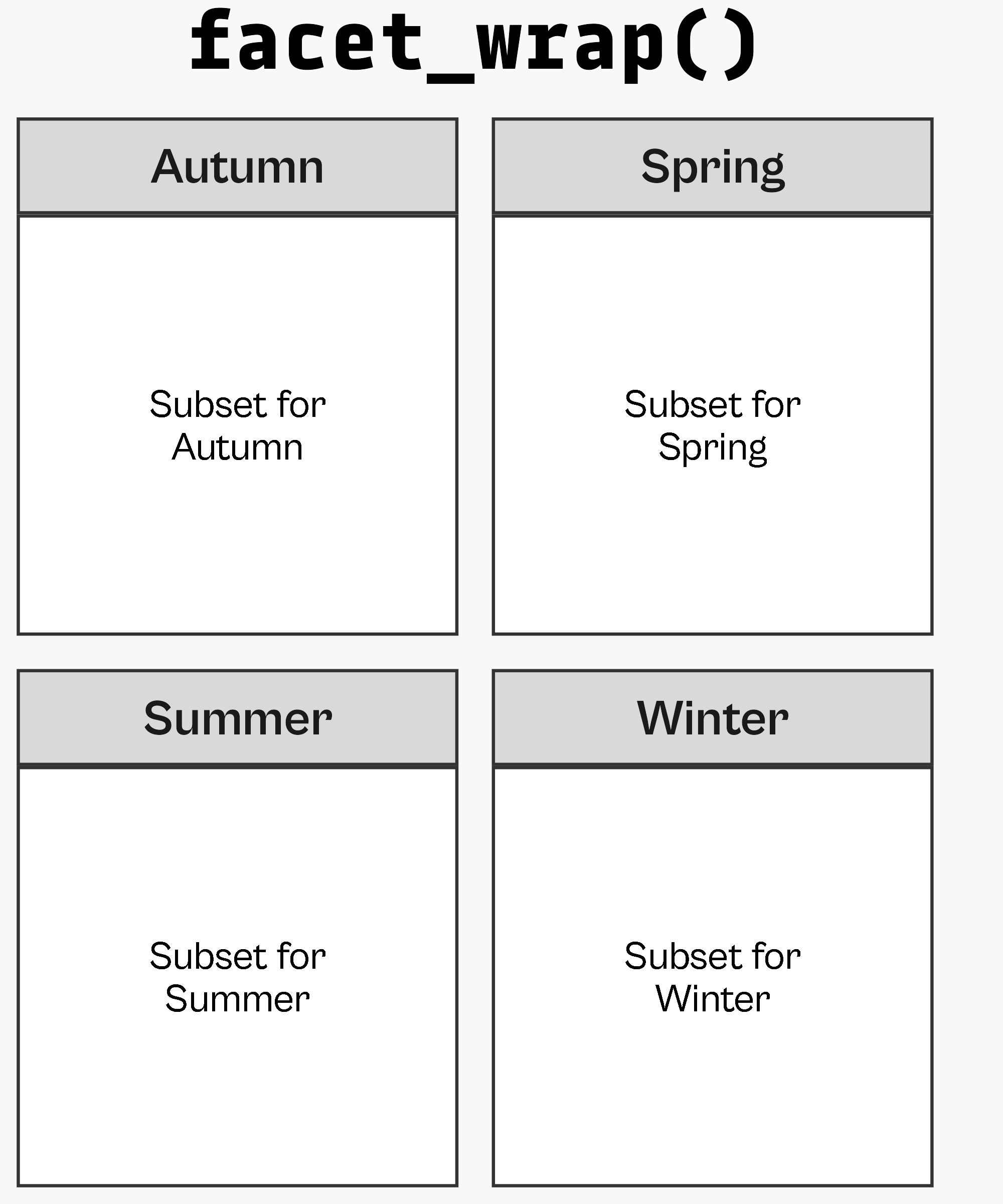
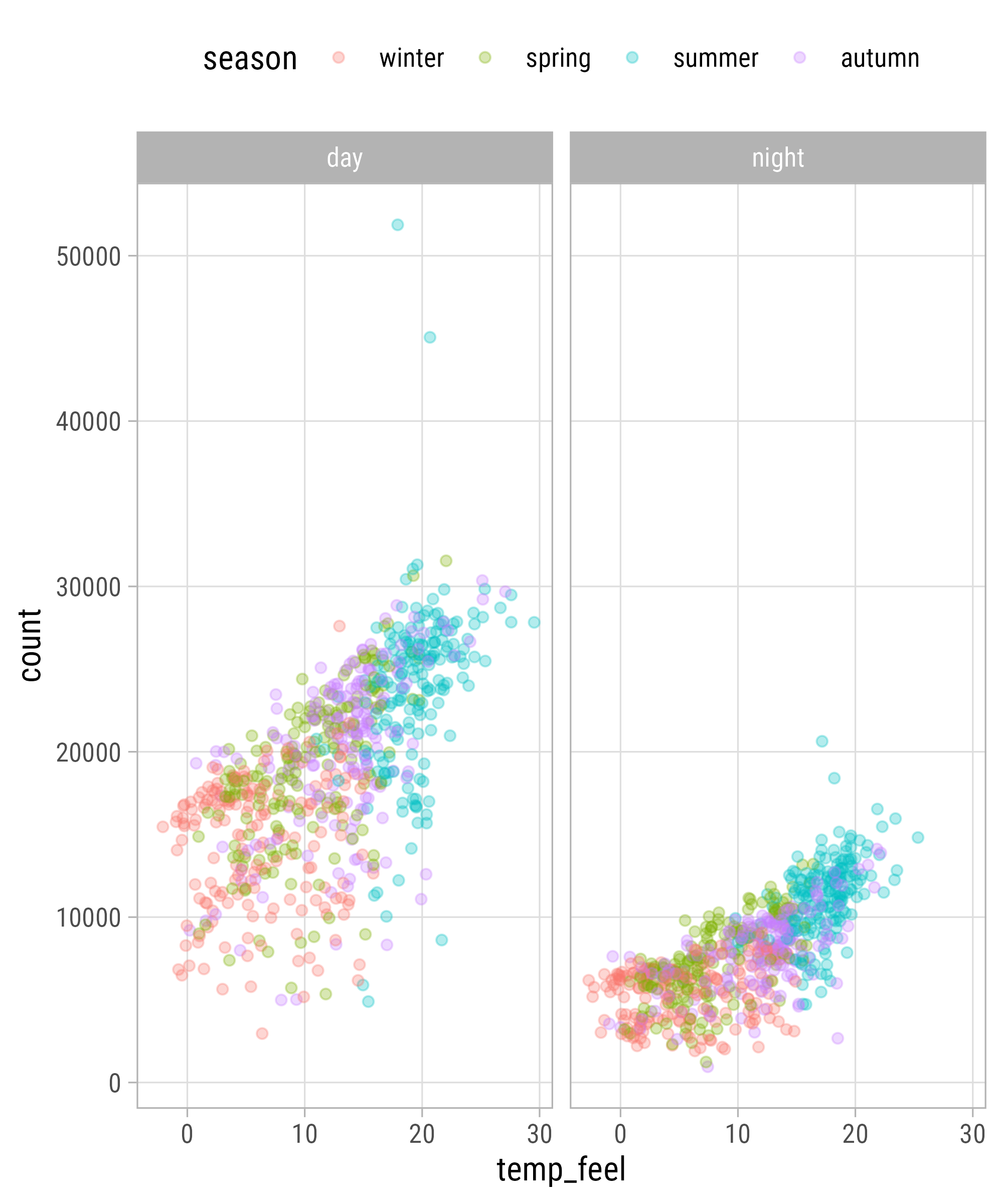
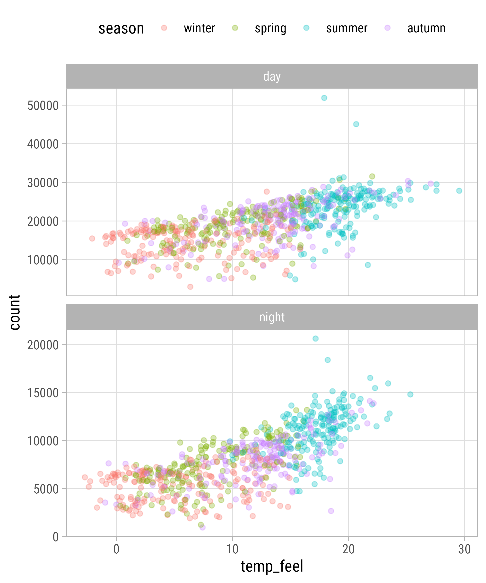
Wrapped Facets

Wrapped Facets
Facet Multiple Variables
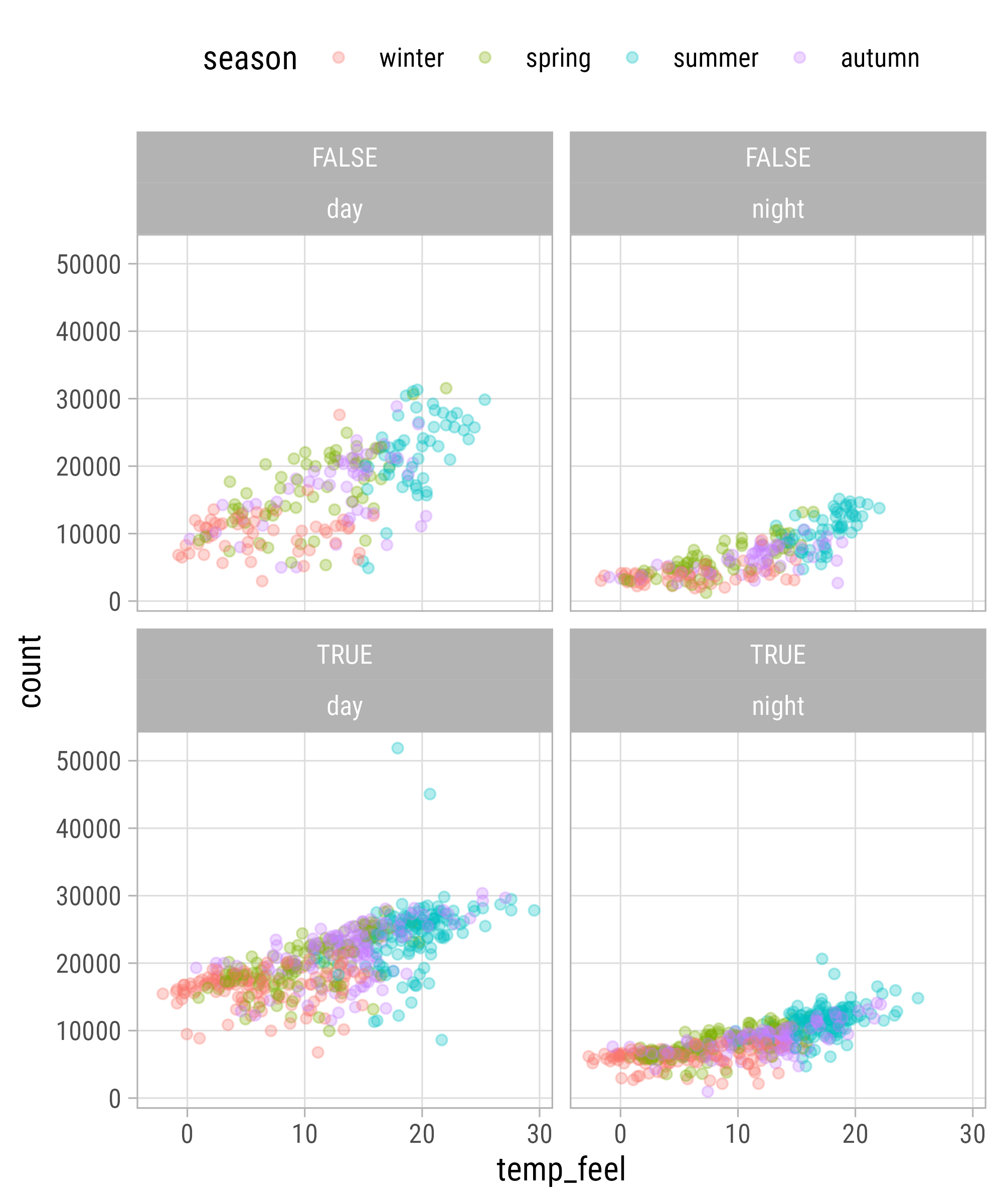
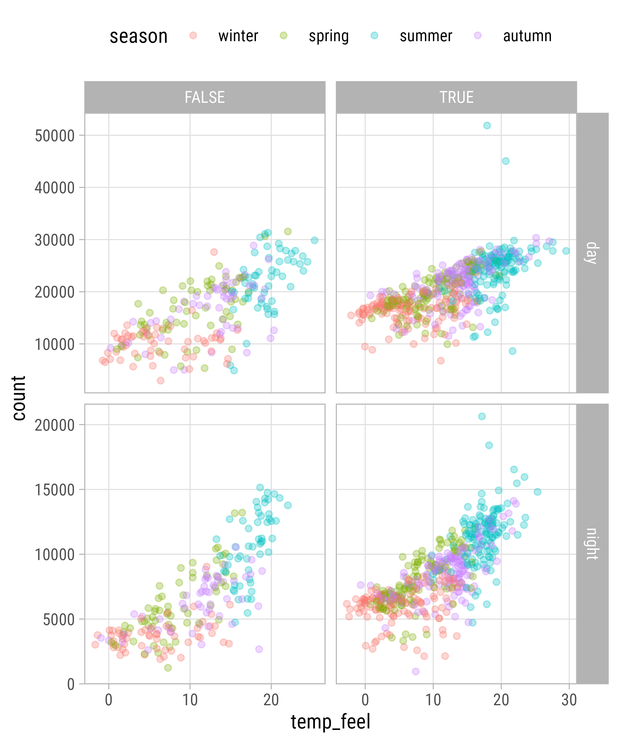
Facet Options: Cols + Rows
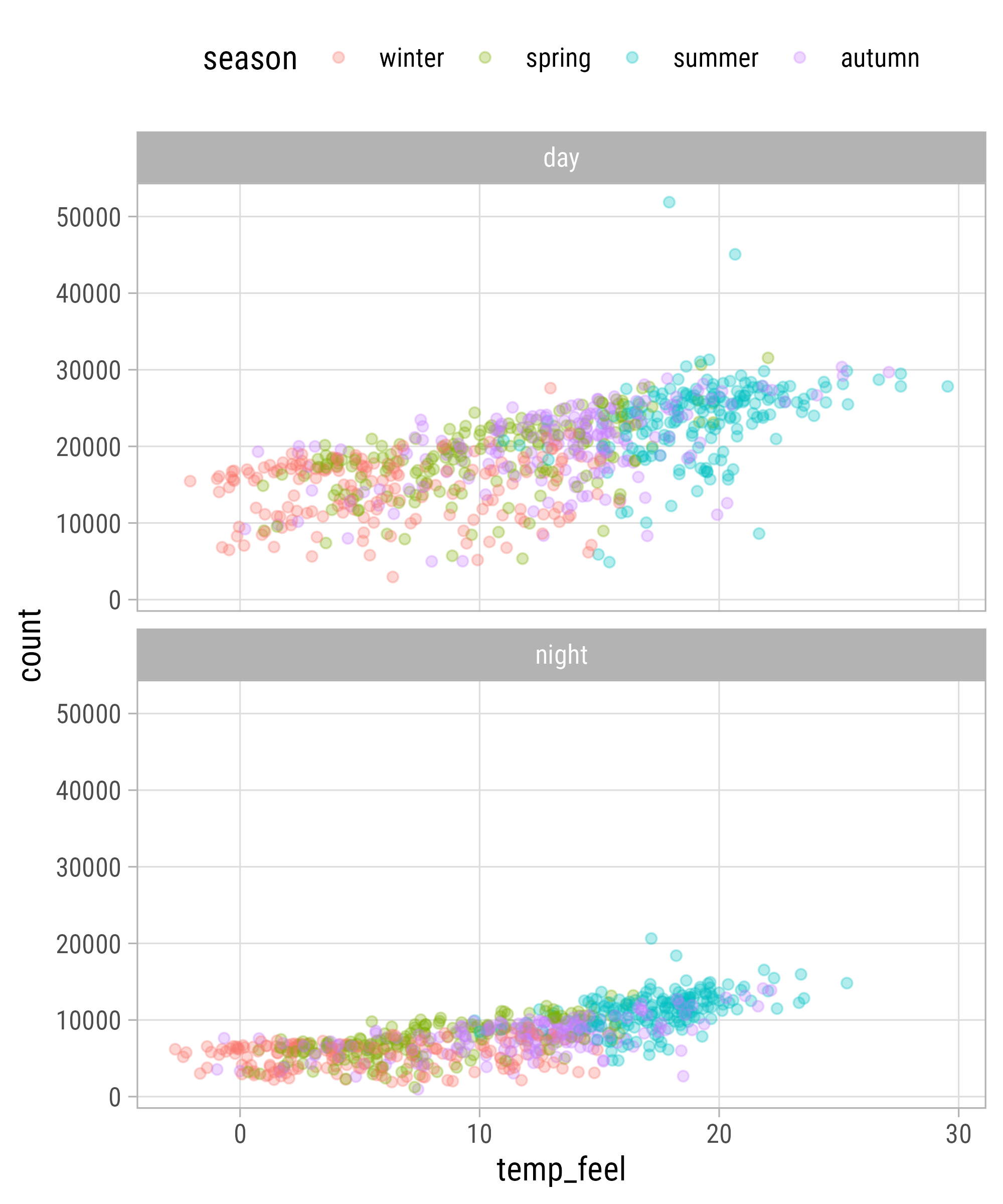
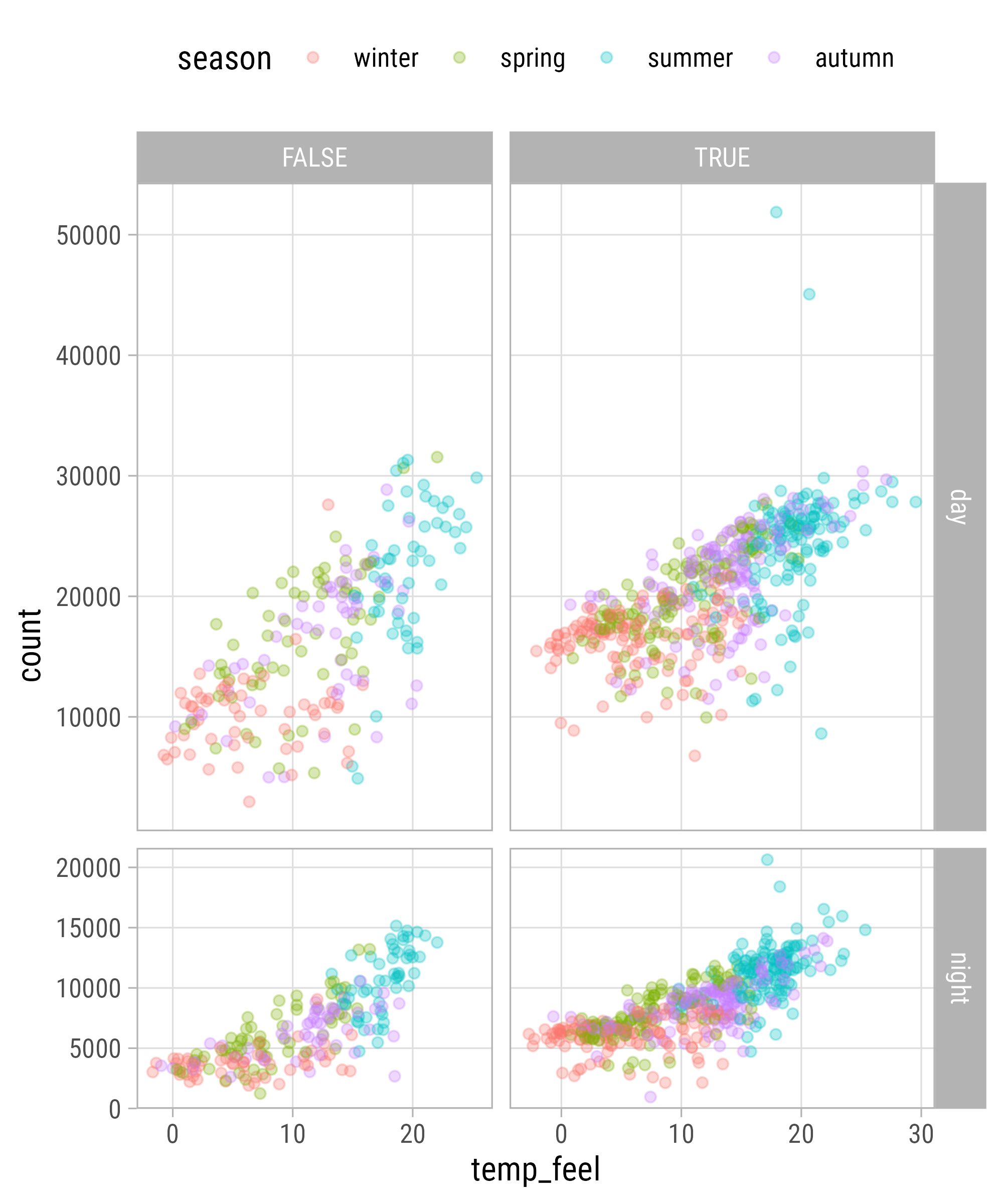
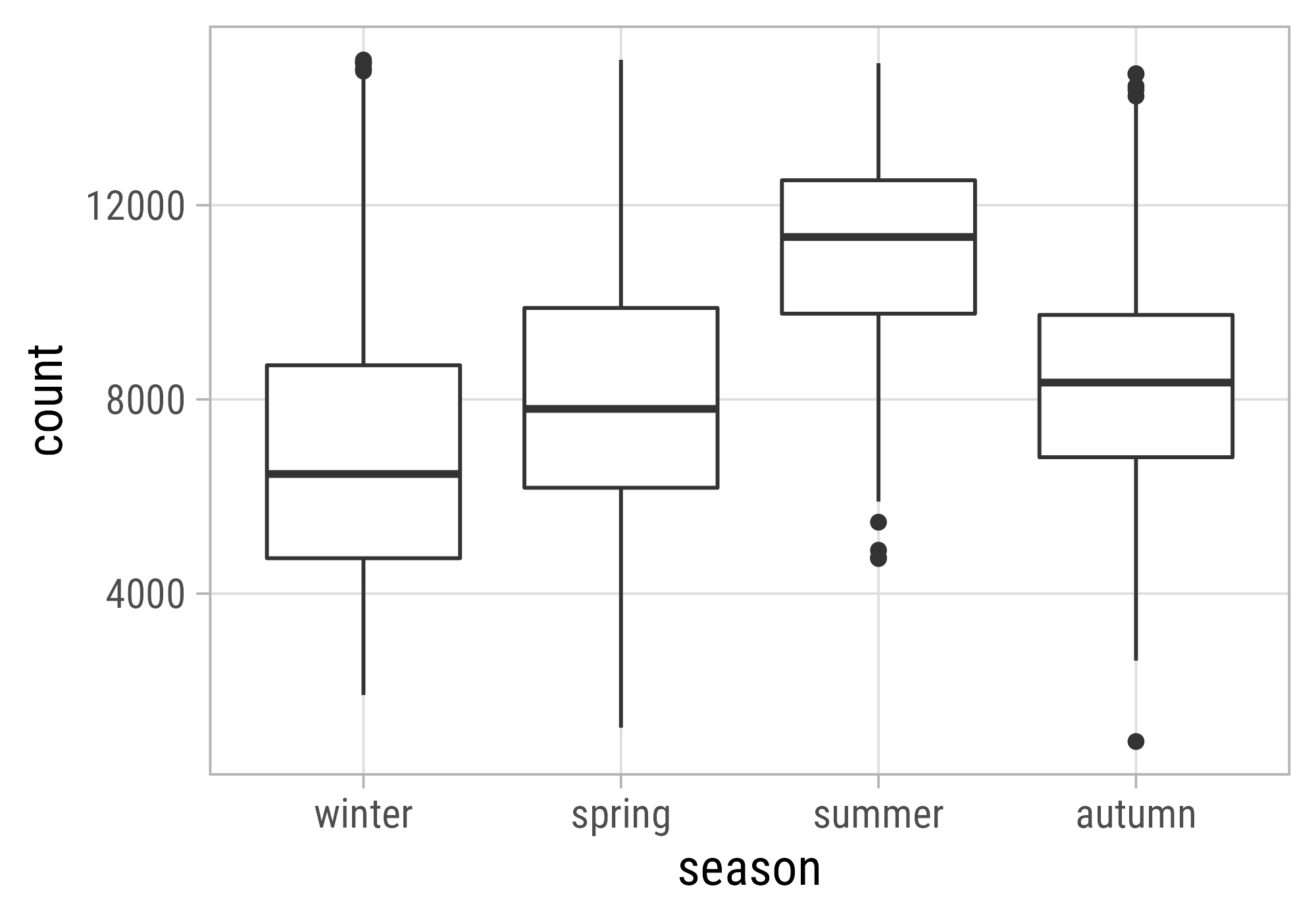
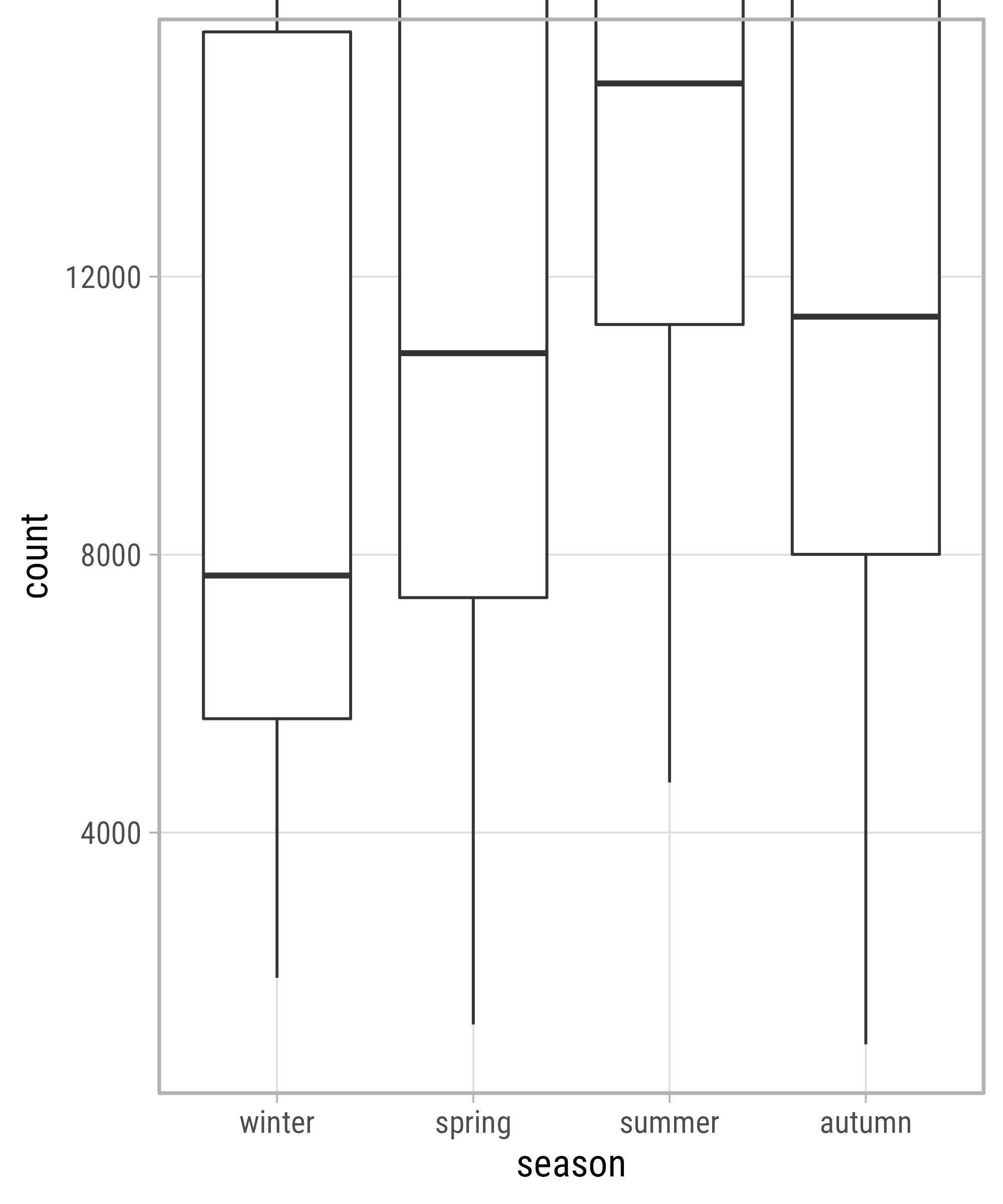
Facet Options: Free Scaling
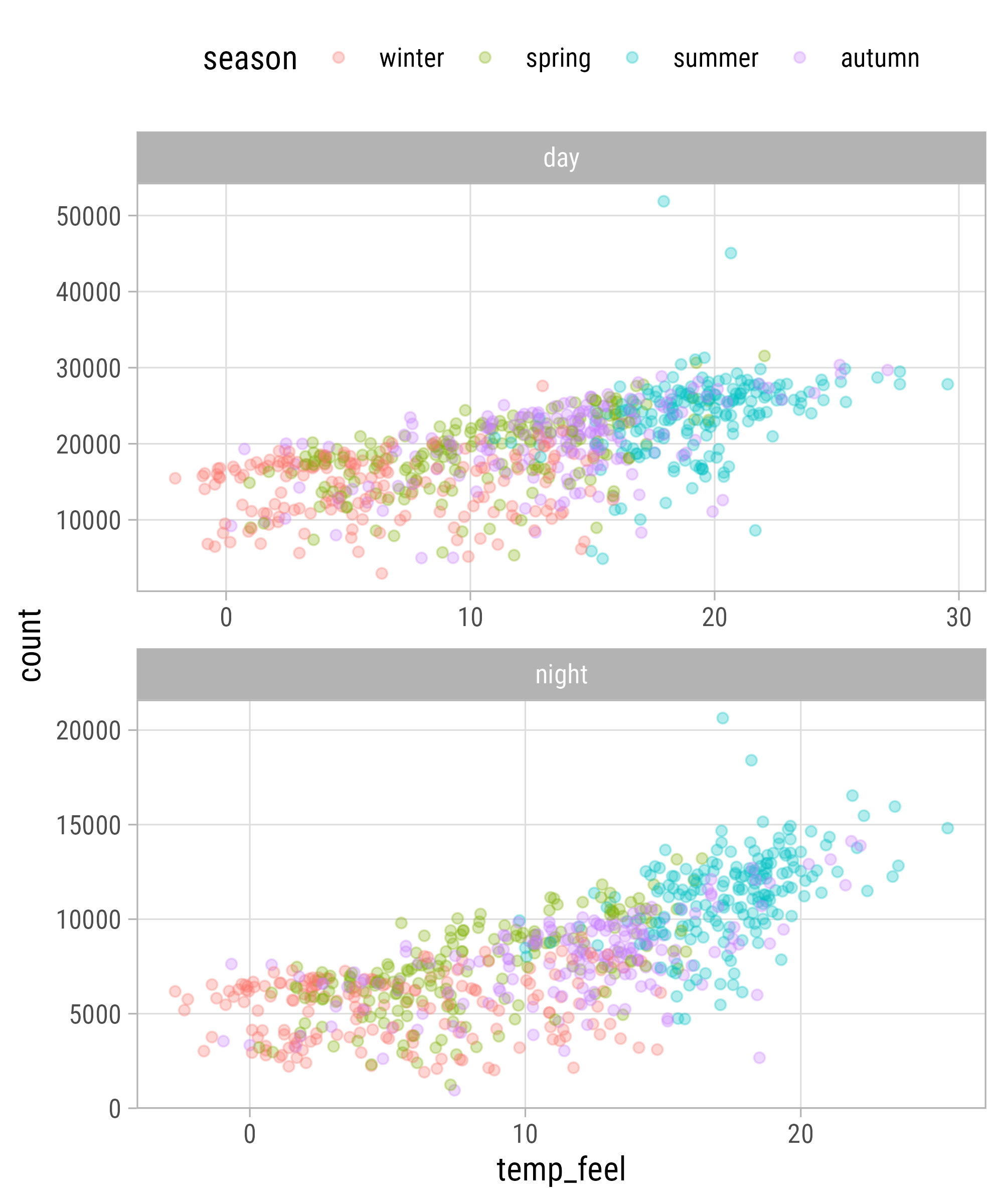
Facet Options: Free Scaling
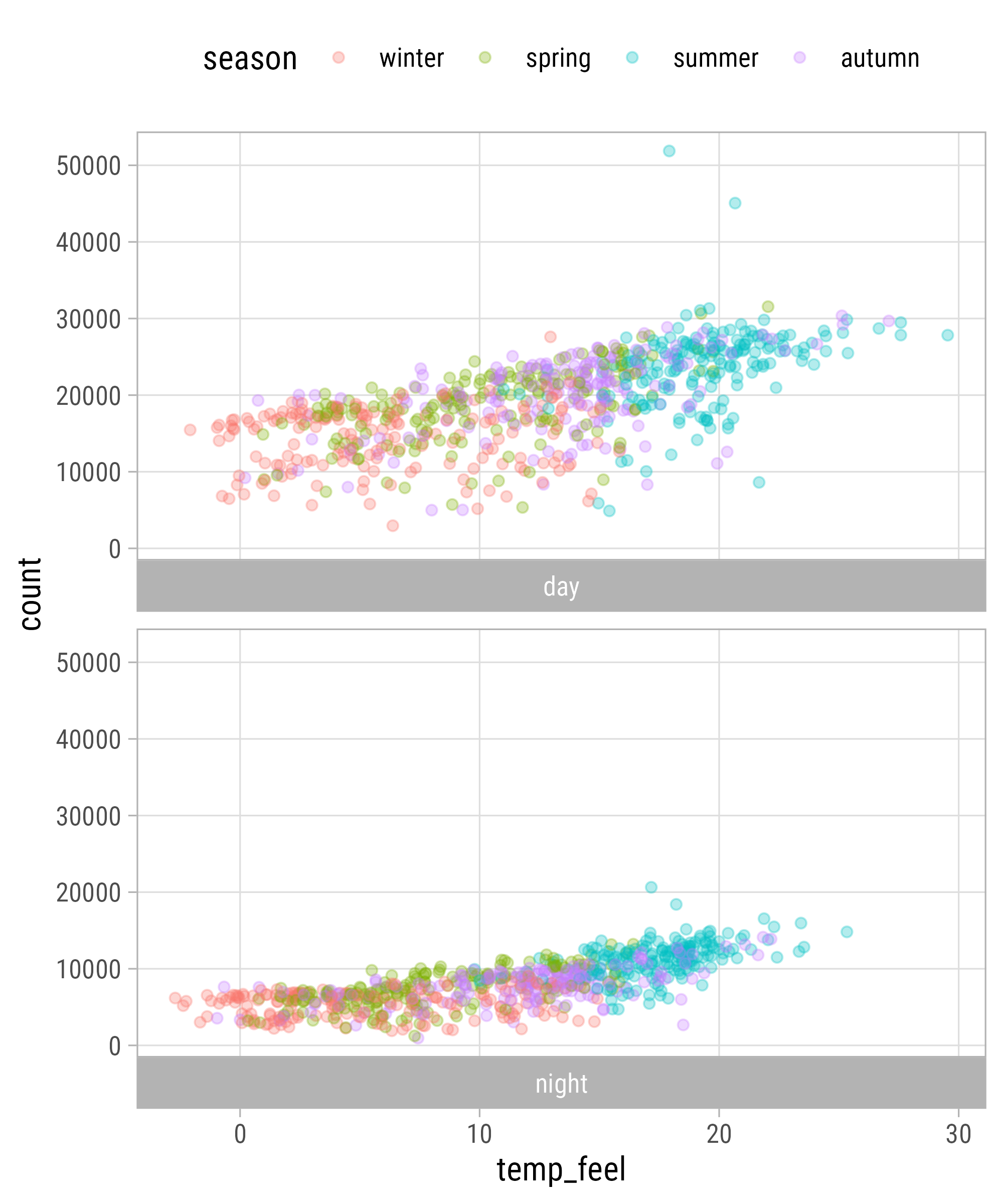
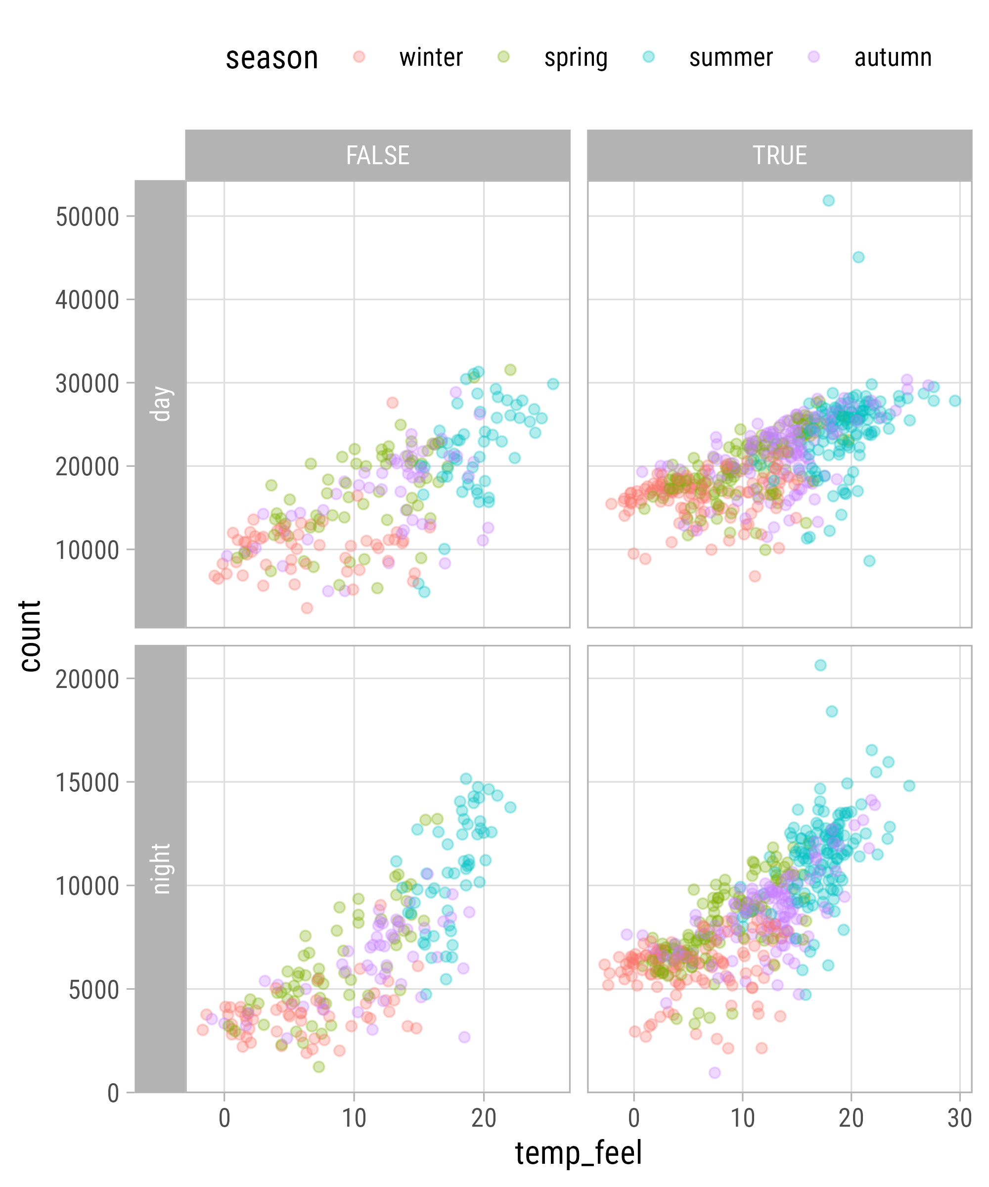
Facet Options: Switch Labels
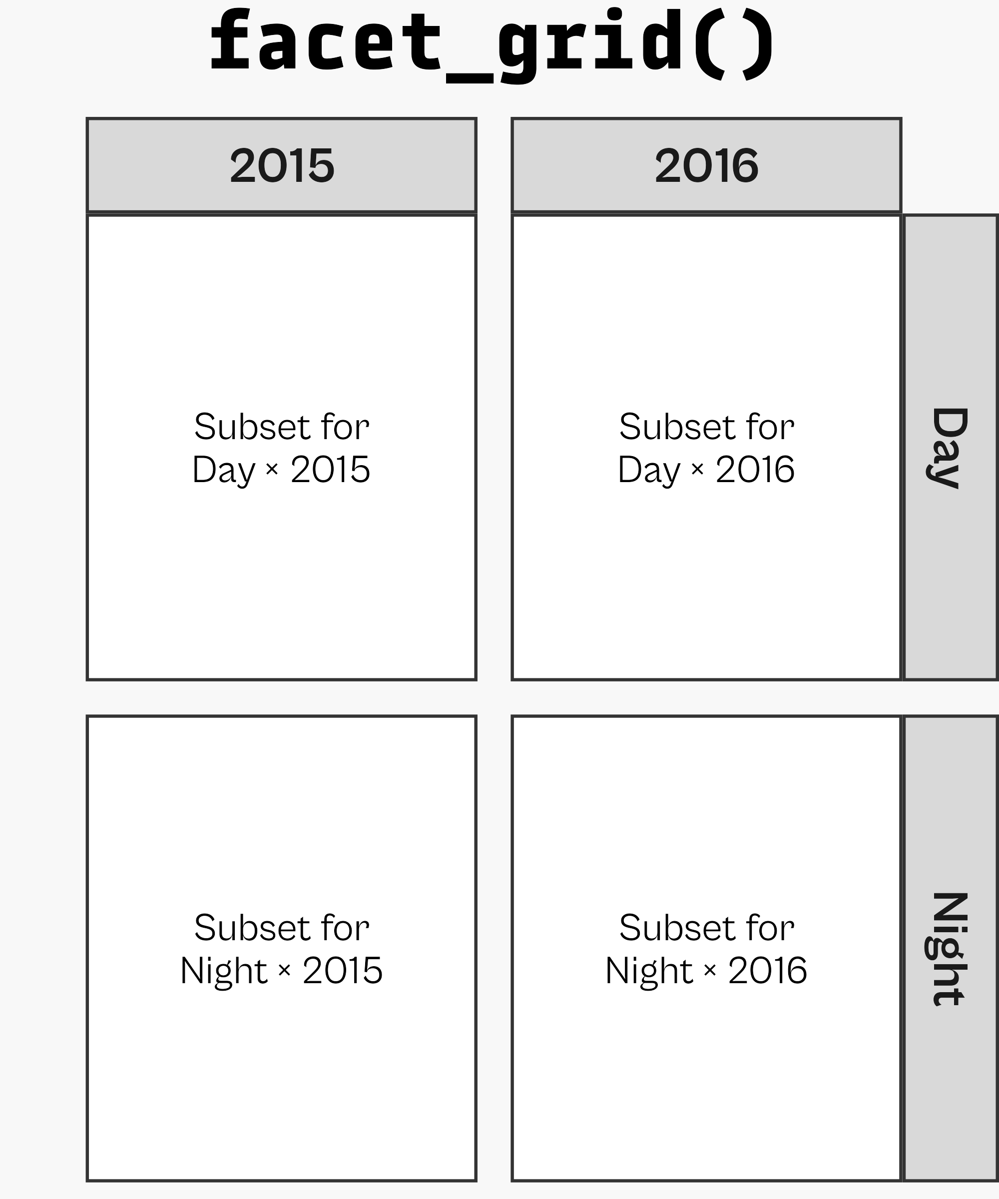
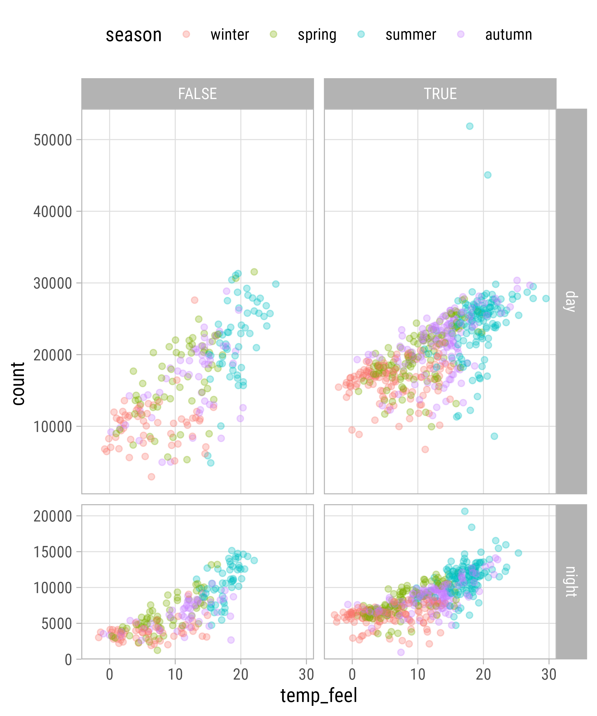
Gridded Facets

Gridded Facets
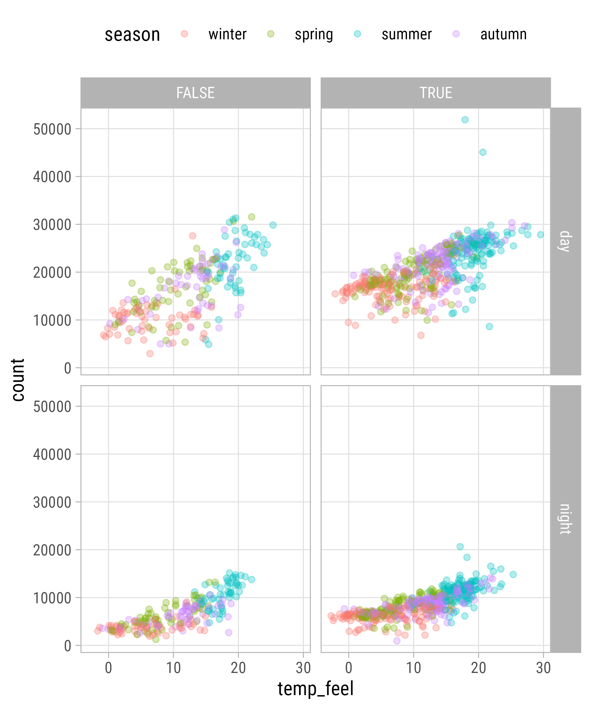
Facet Multiple Variables
Facet Options: Free Scaling
Facet Options: Switch Labels
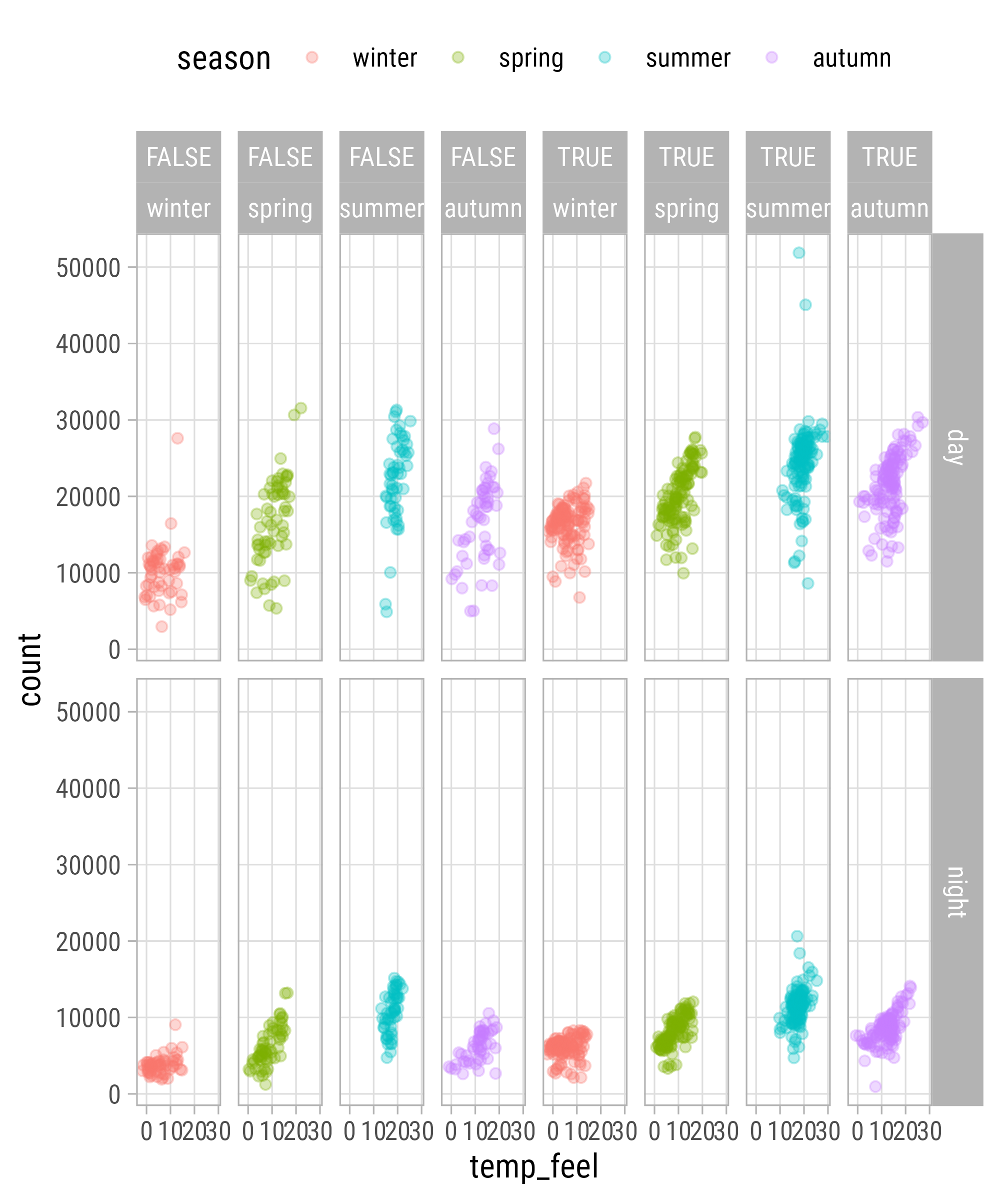
Facet Options: Proportional Spacing
Facet Options: Proportional Spacing
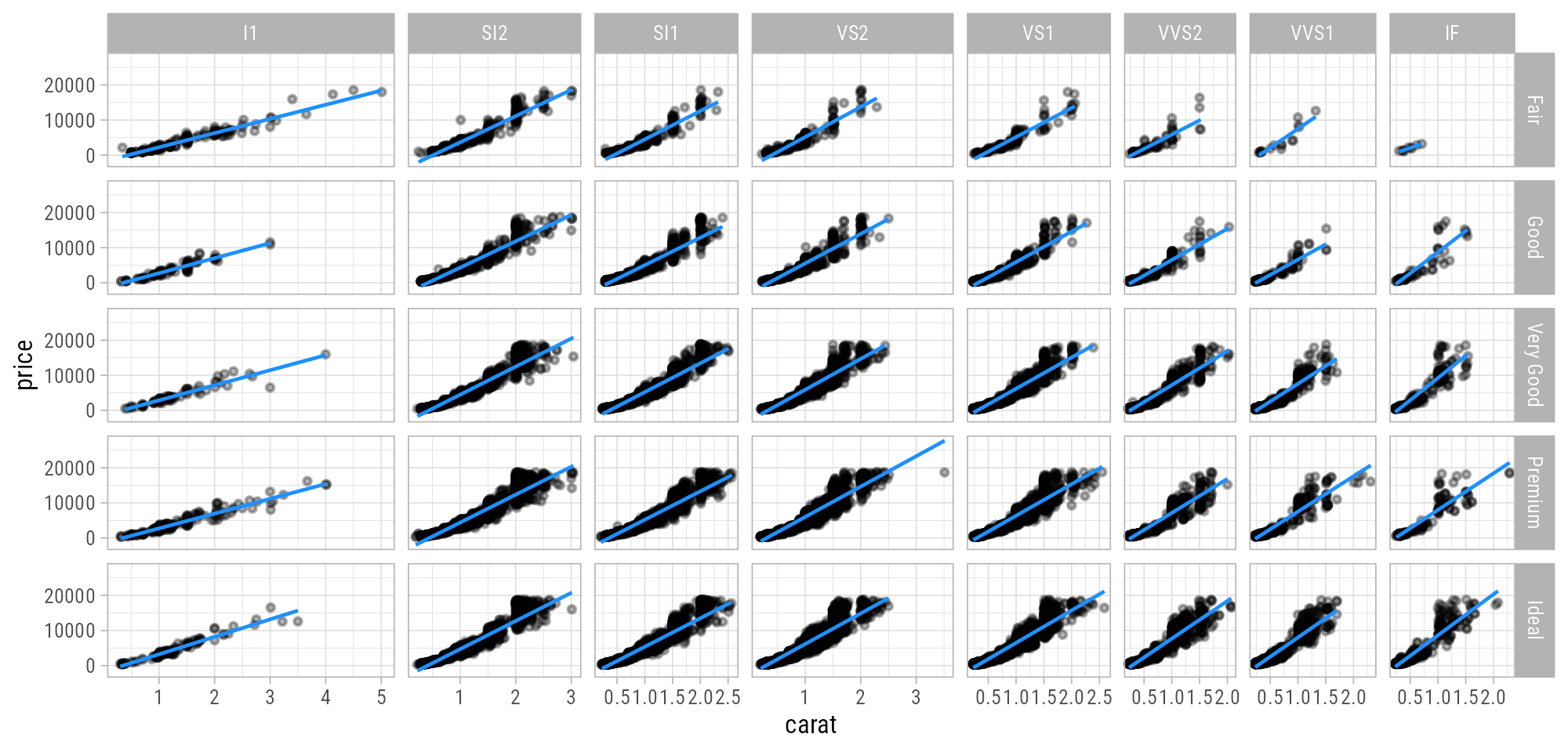
Your Turn!
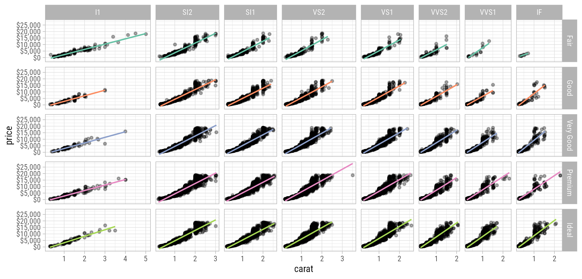
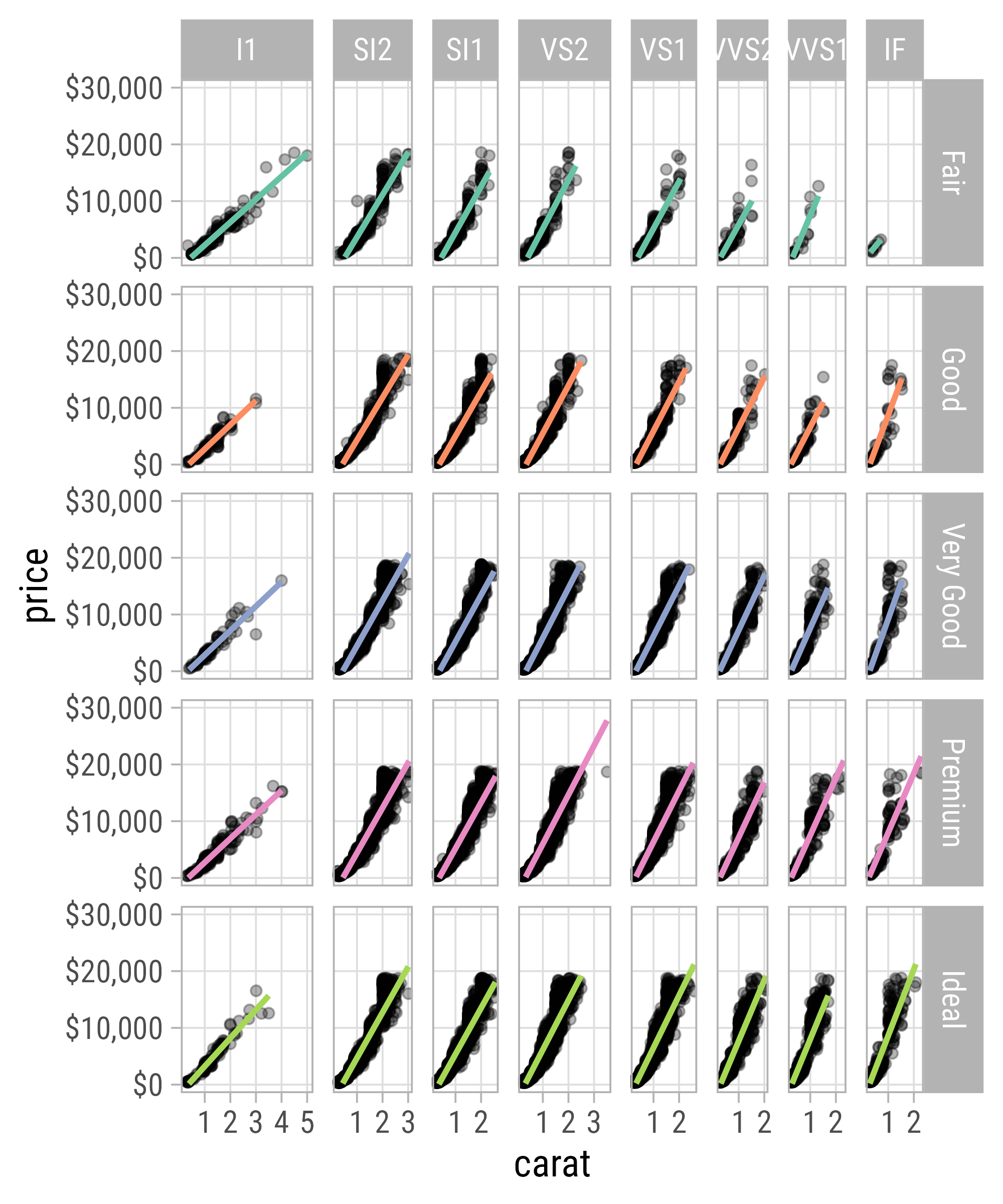
Create the following facet from the diamonds data.
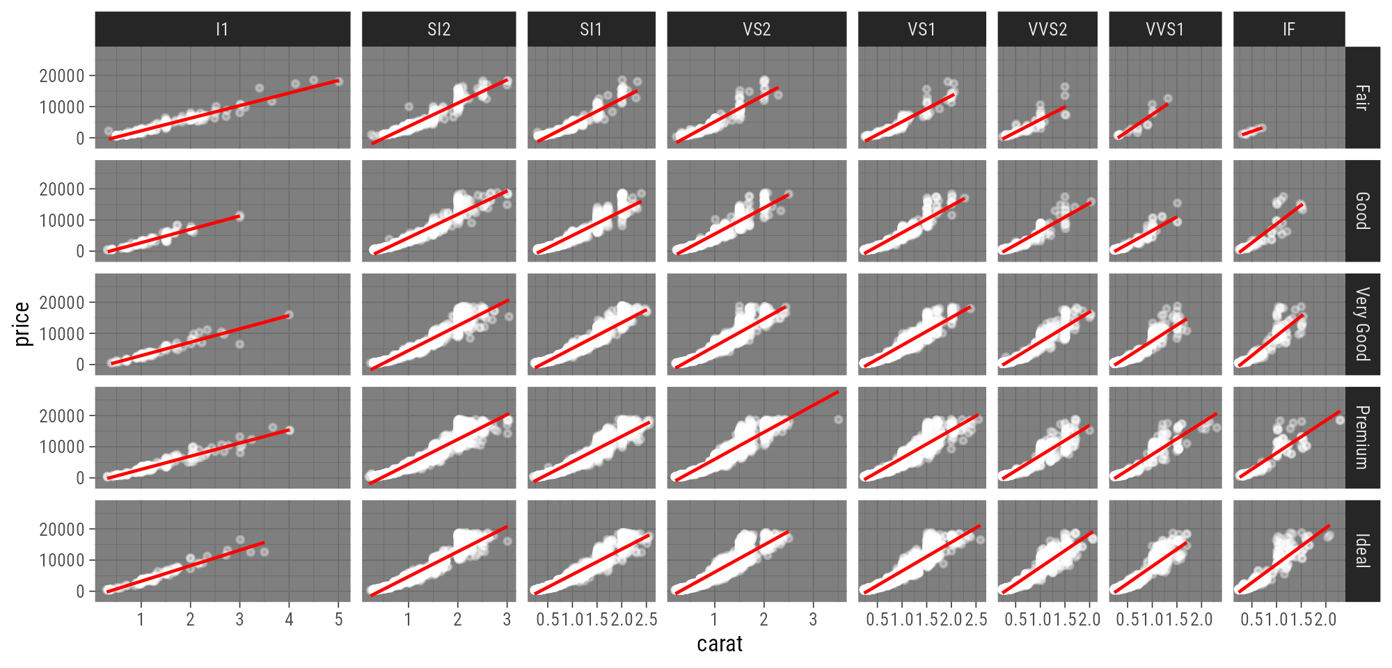
Your Turn!
Bonus: Create this bloody-dark version.
Diamonds Facet
Diamonds Facet
Diamonds Facet (Dark Theme Bonus)
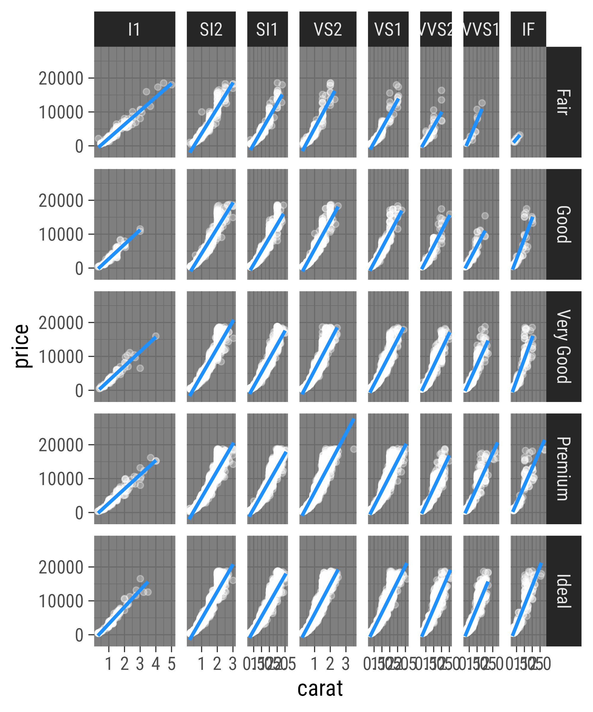
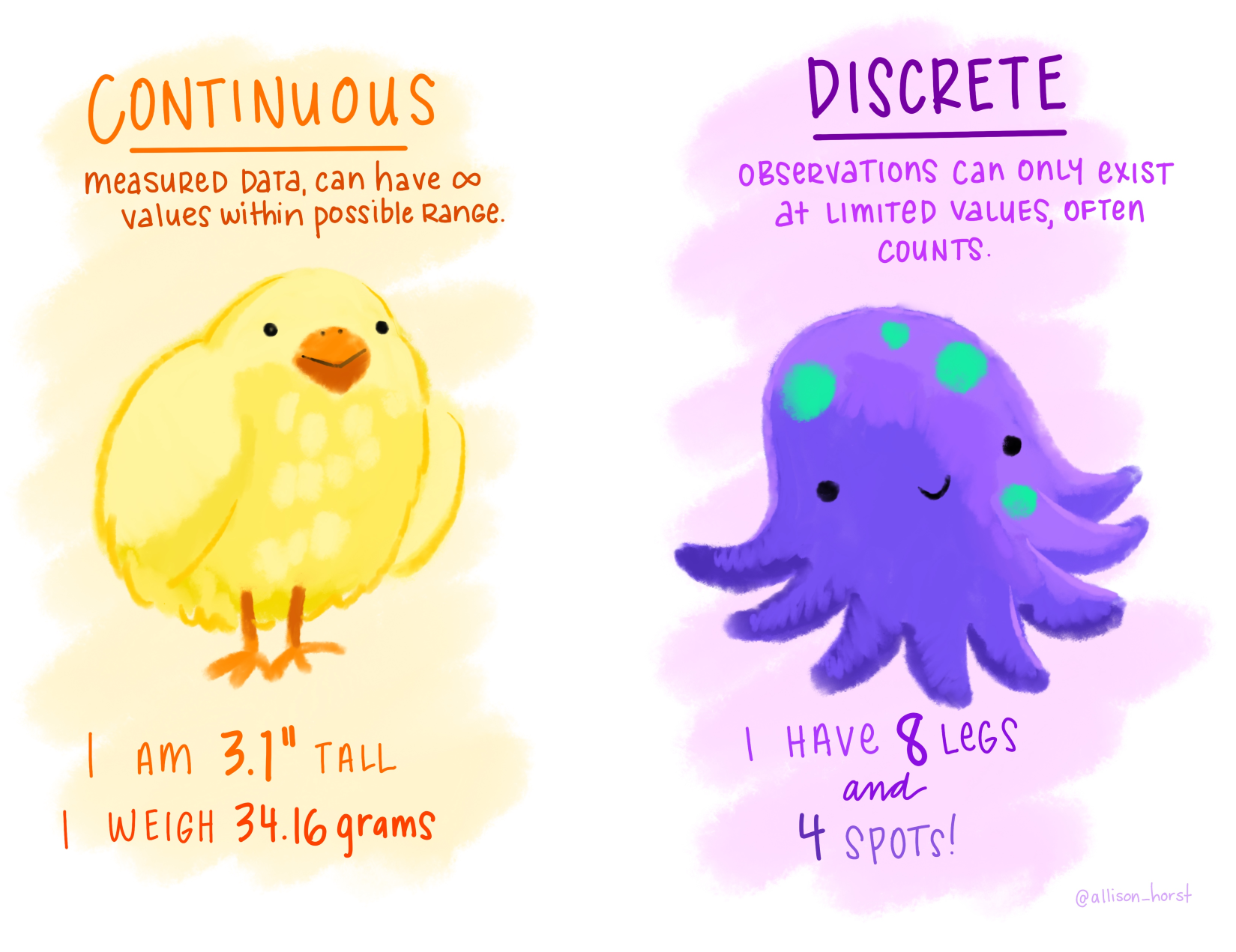
Illustration by Allison Horst
Aesthetics + Scales

Aesthetics + Scales
Scales

Scales
Scales
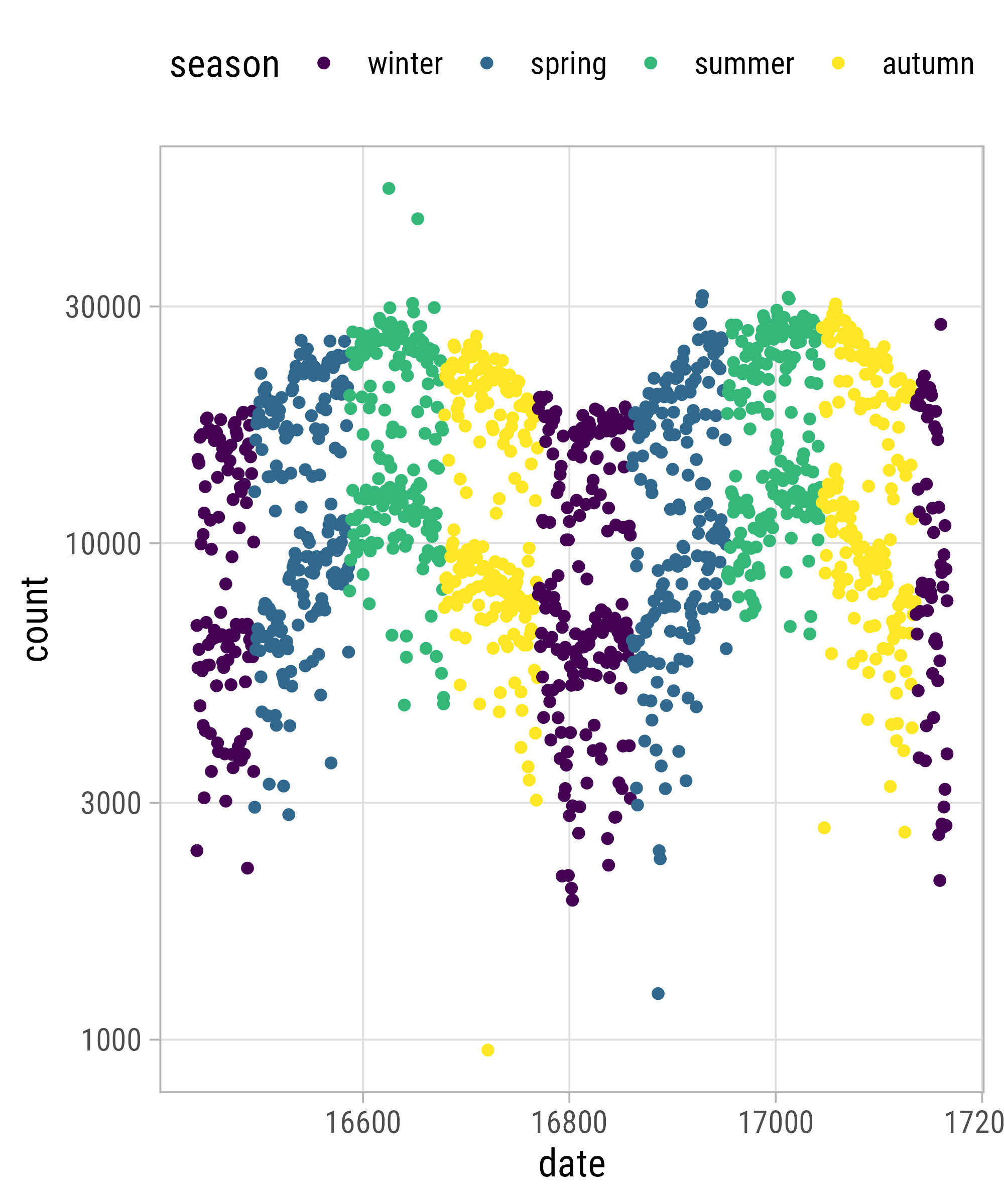
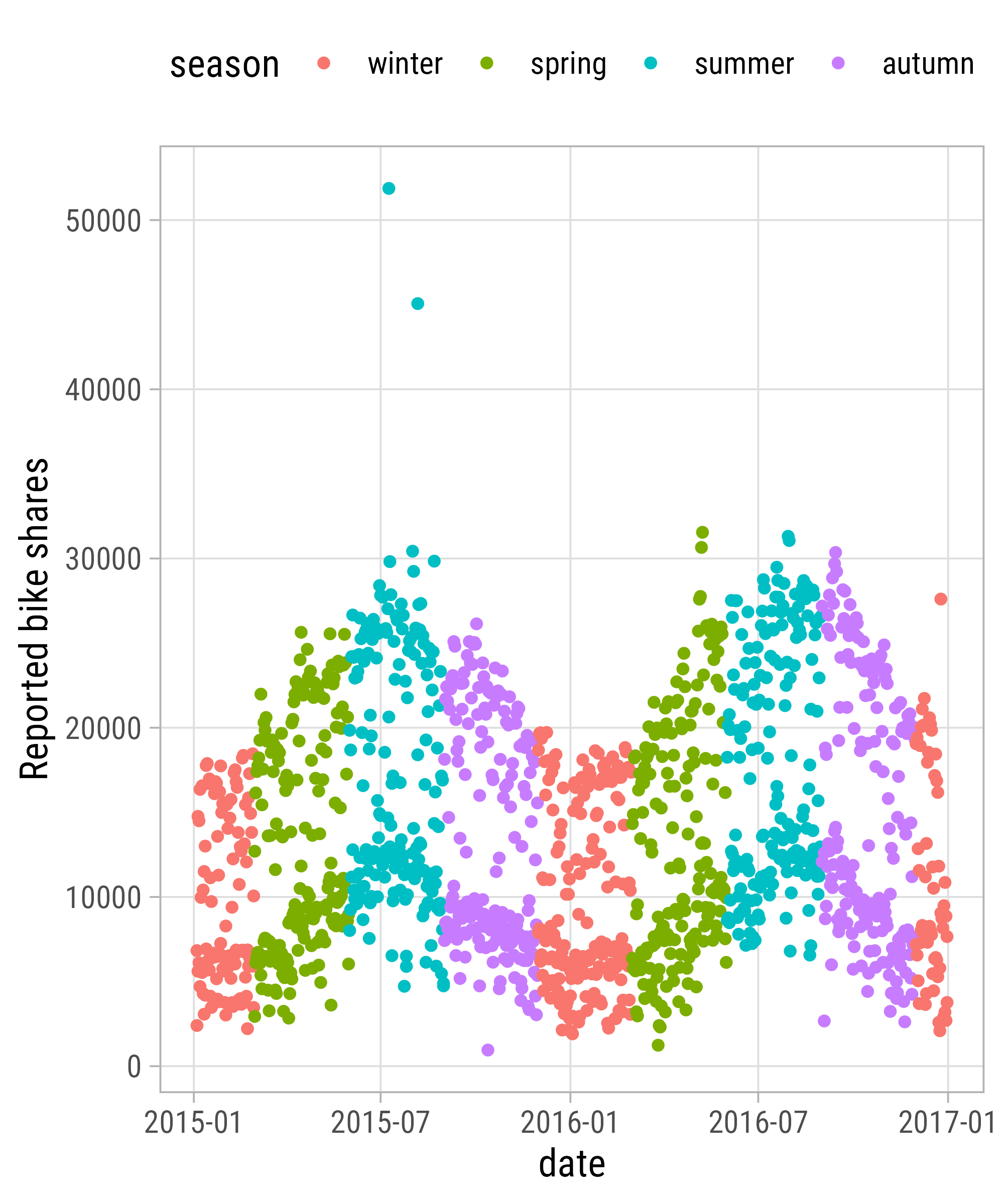
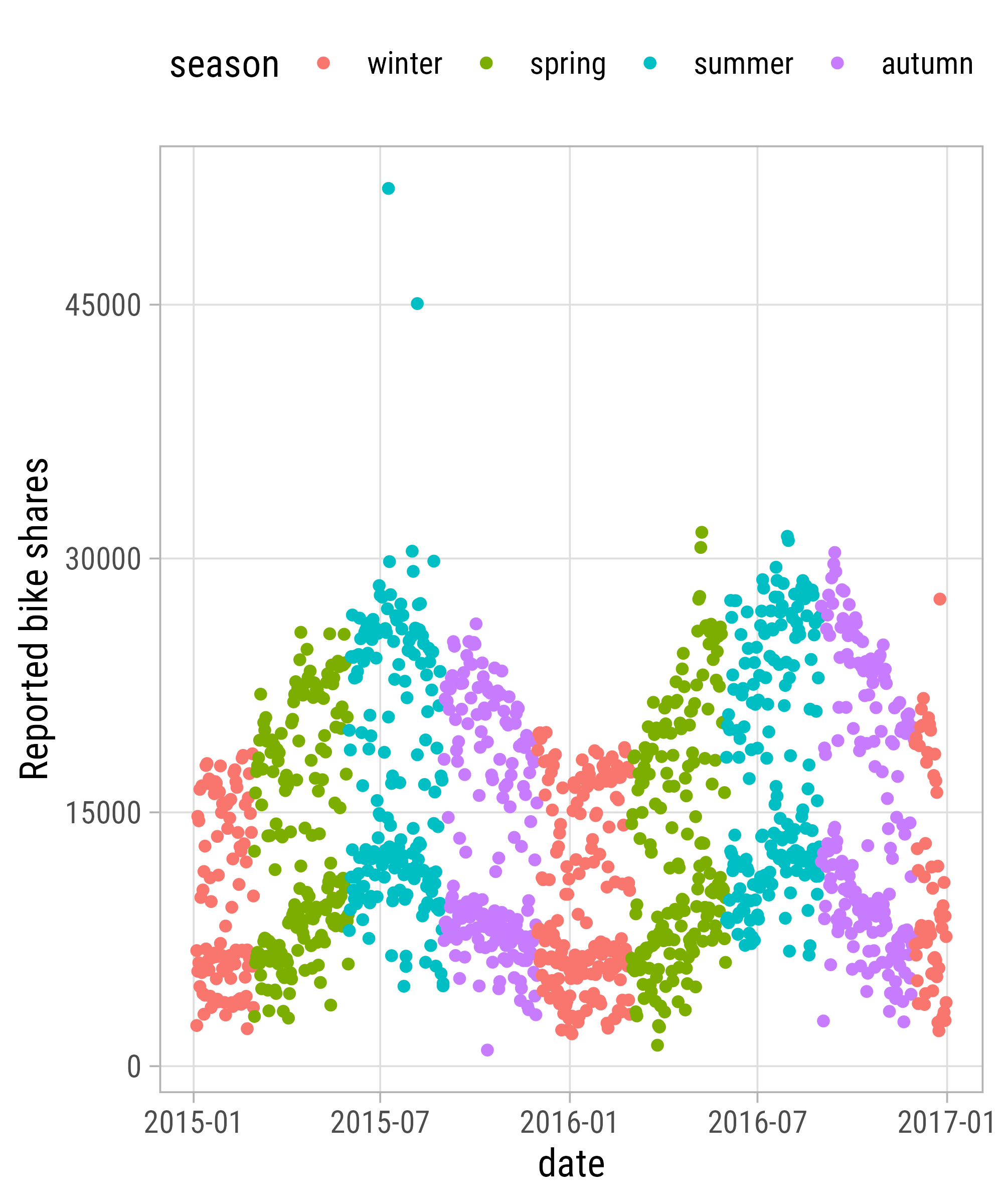
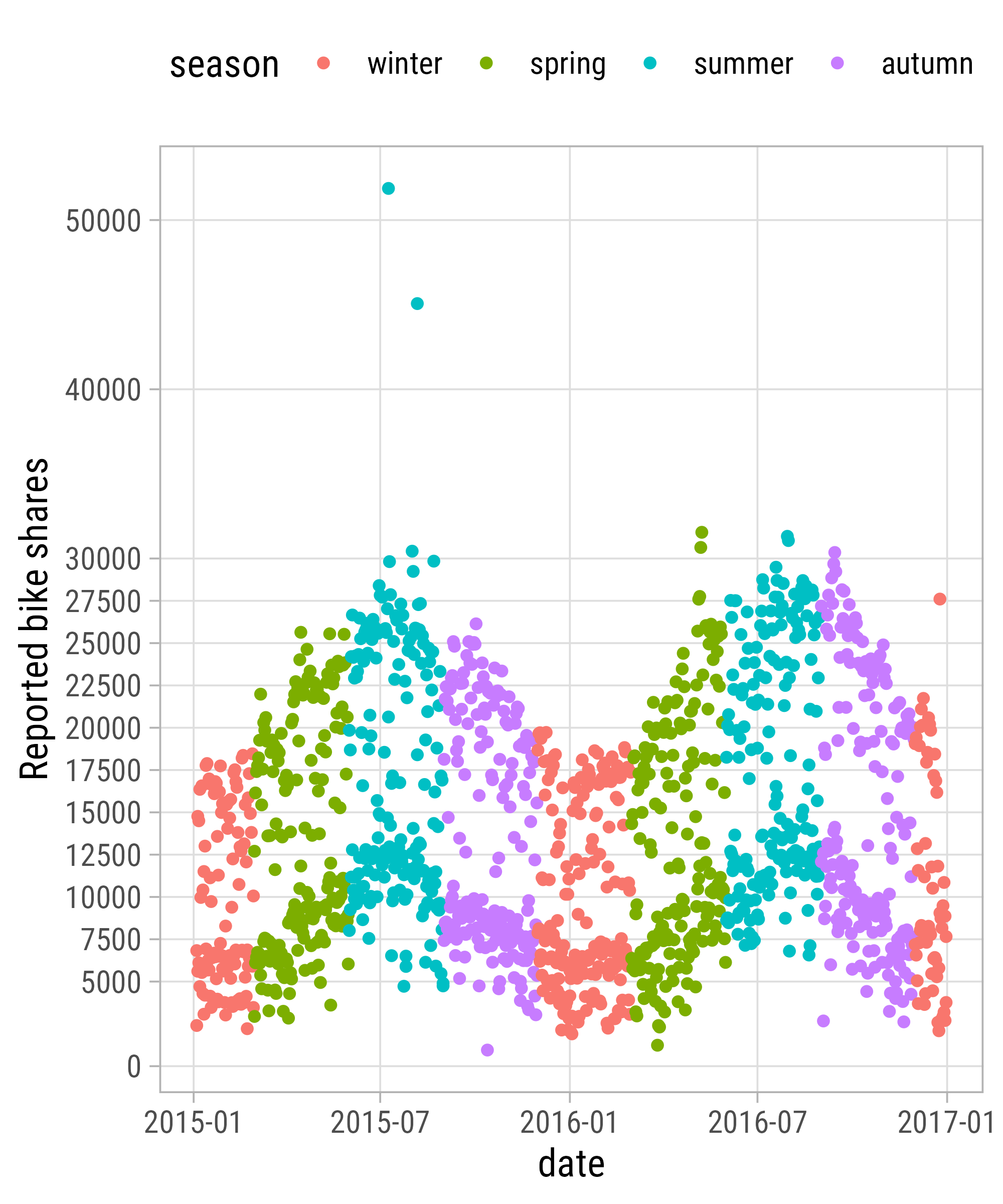
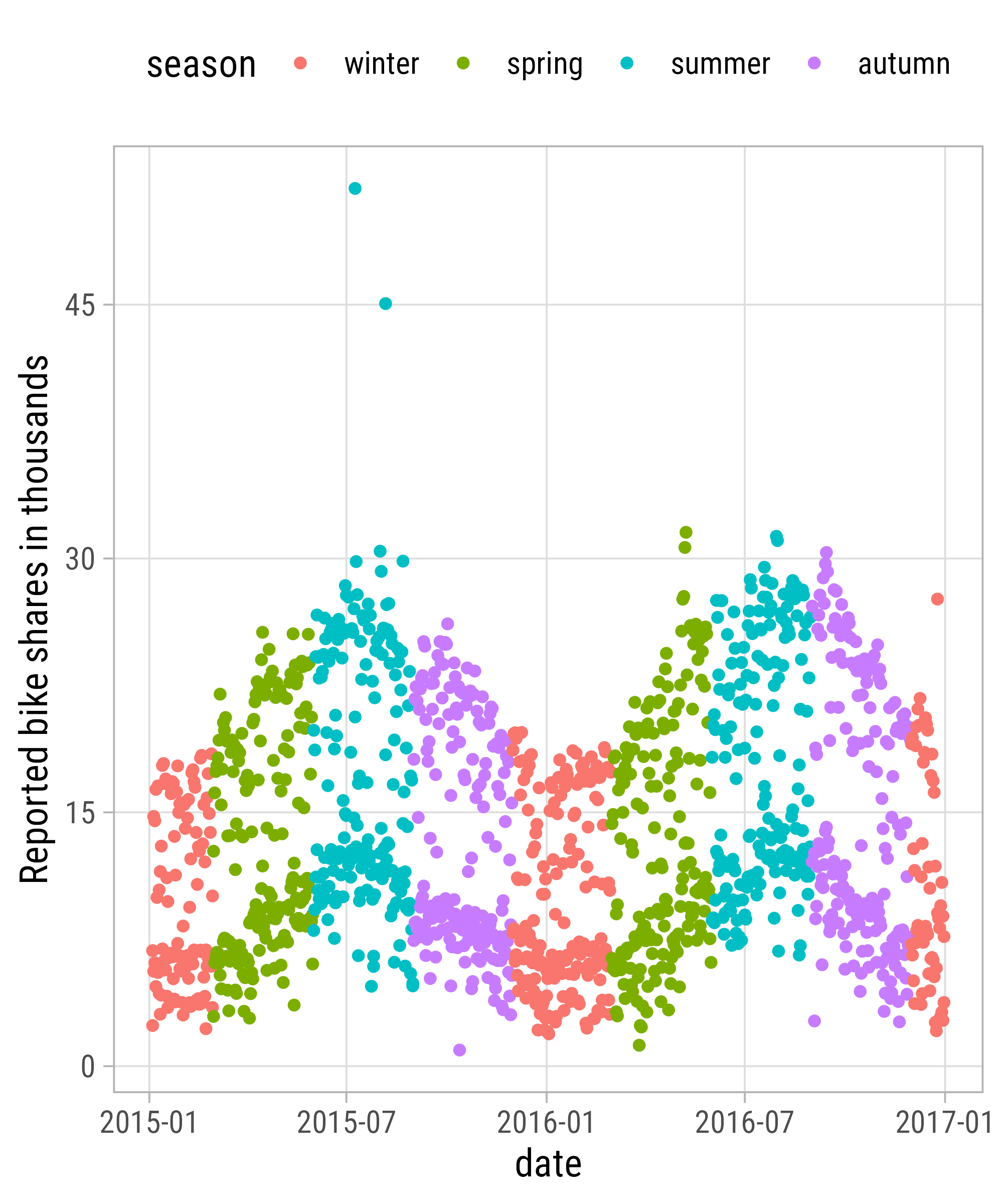
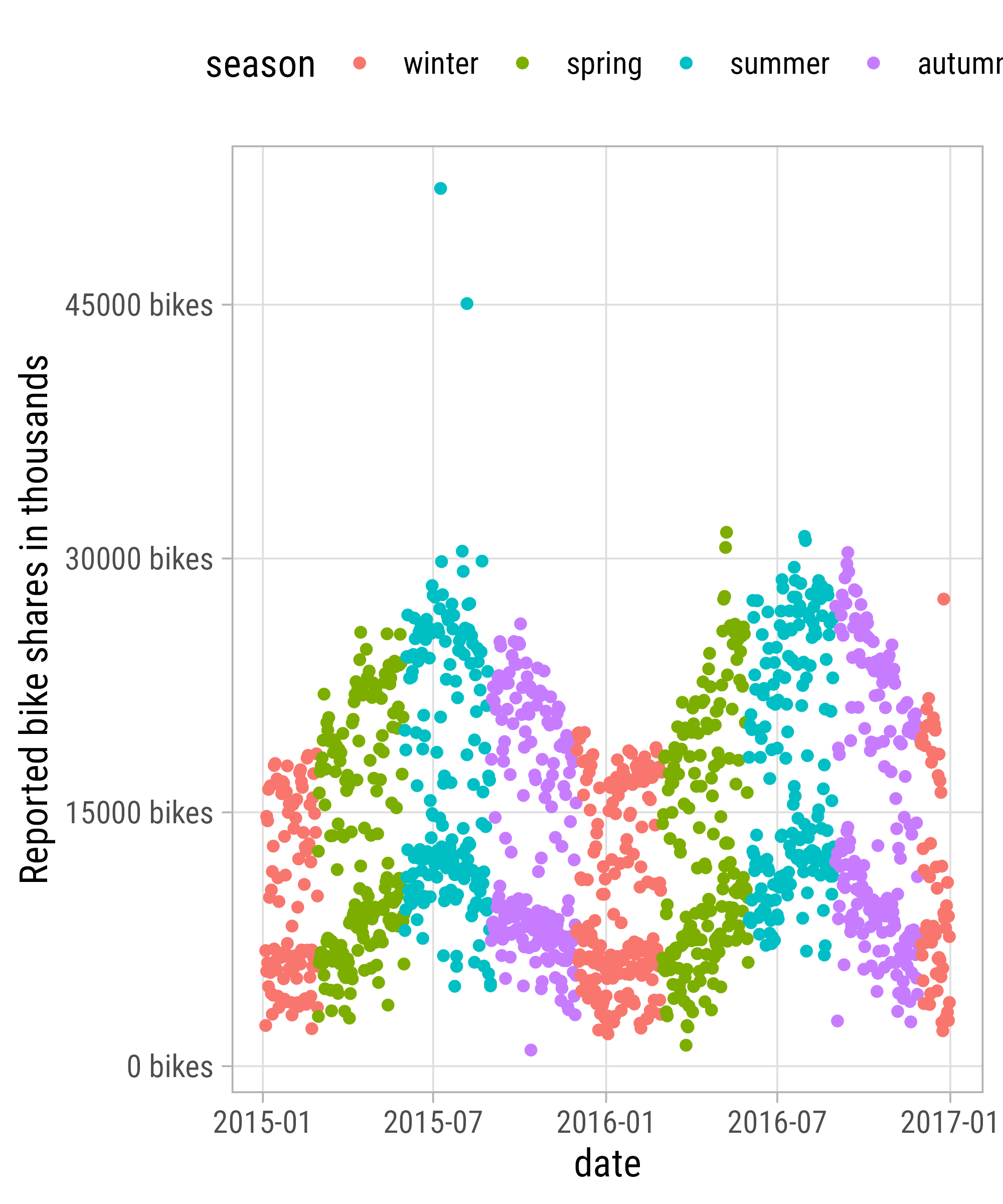
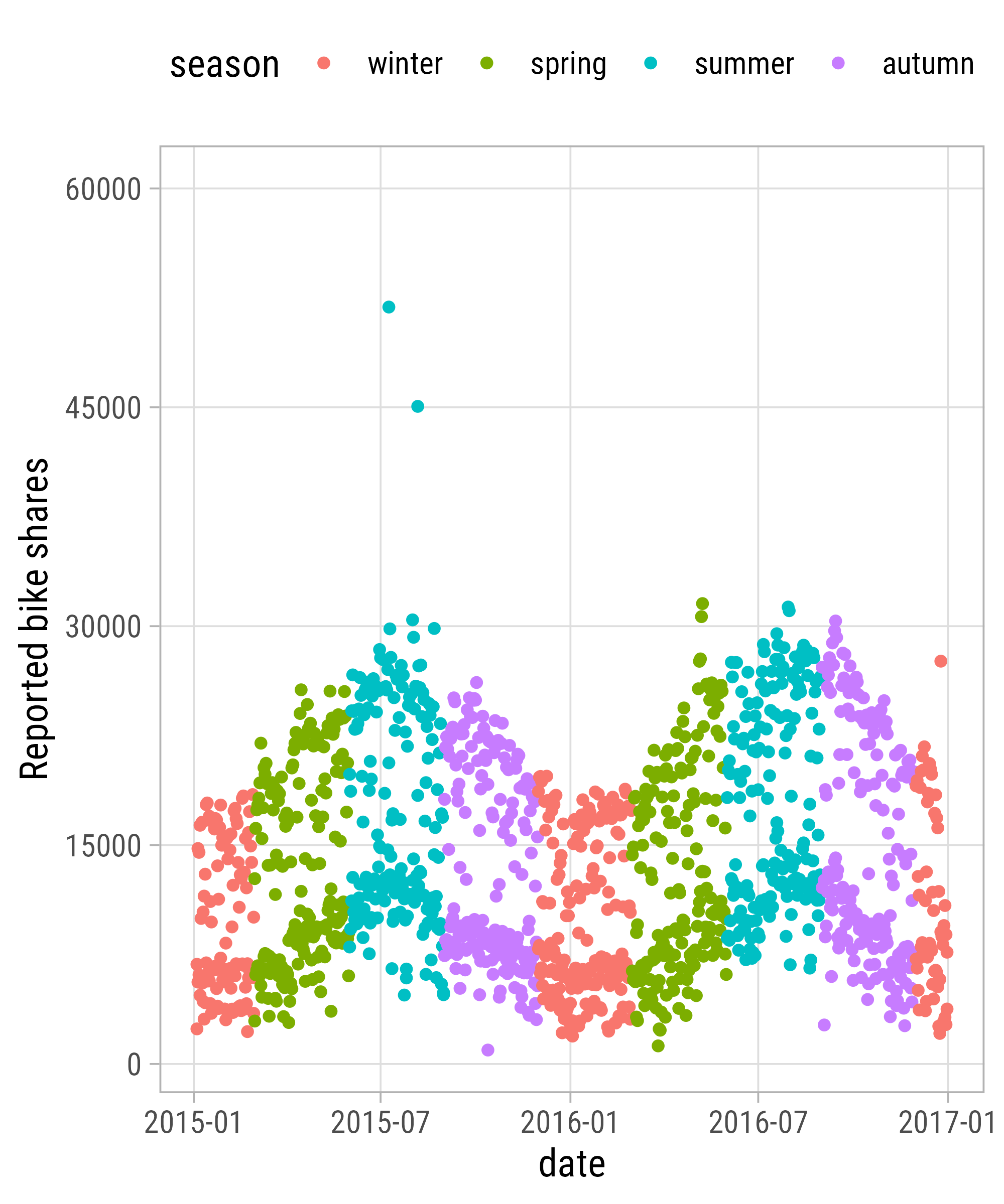
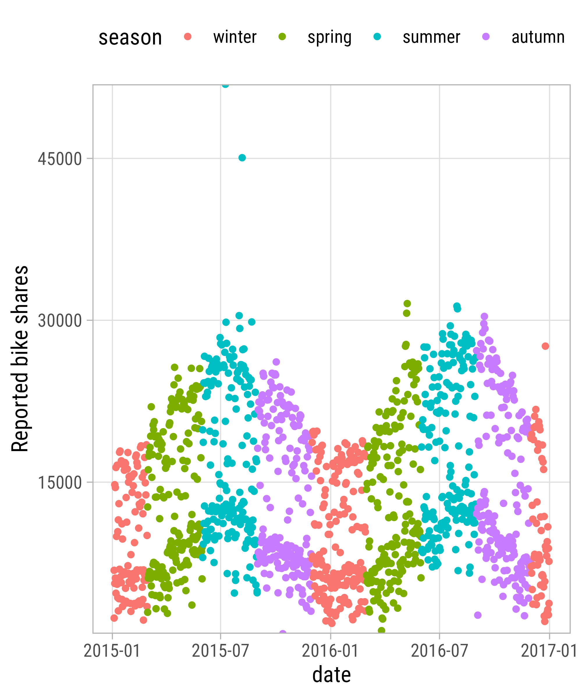
`scale_x|y_continuous`
`scale_x|y_continuous`
`scale_x|y_continuous`
`scale_x|y_continuous`

`scale_x|y_continuous`
`scale_x|y_continuous`
`scale_x|y_continuous`
`scale_x|y_continuous`
`scale_x|y_continuous`
`scale_x|y_continuous`
`scale_x|y_continuous`

`scale_x|y_continuous`
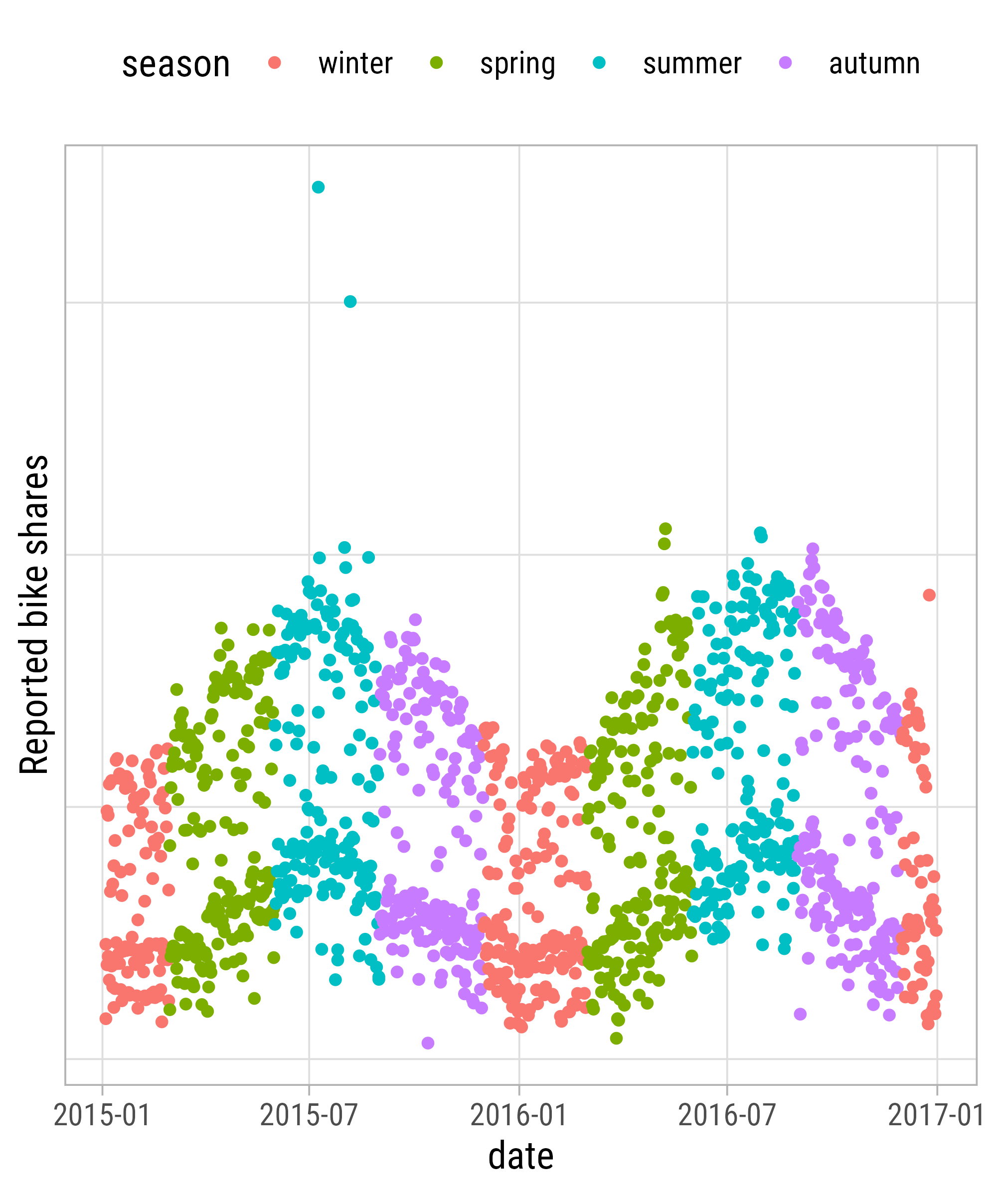
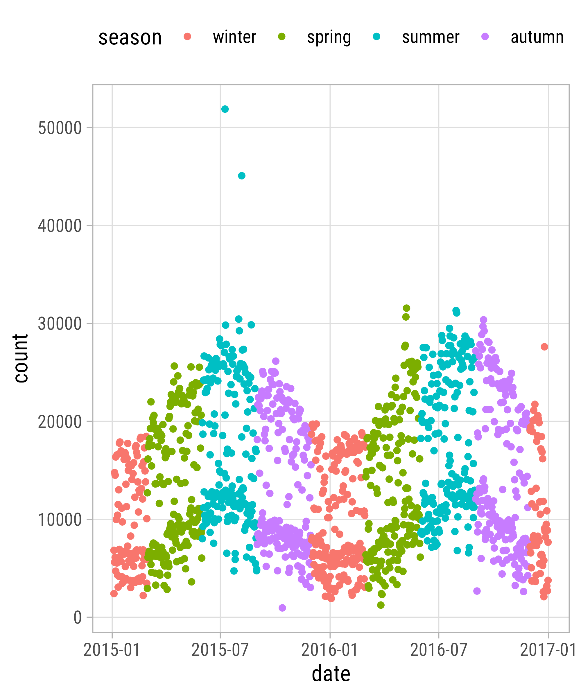
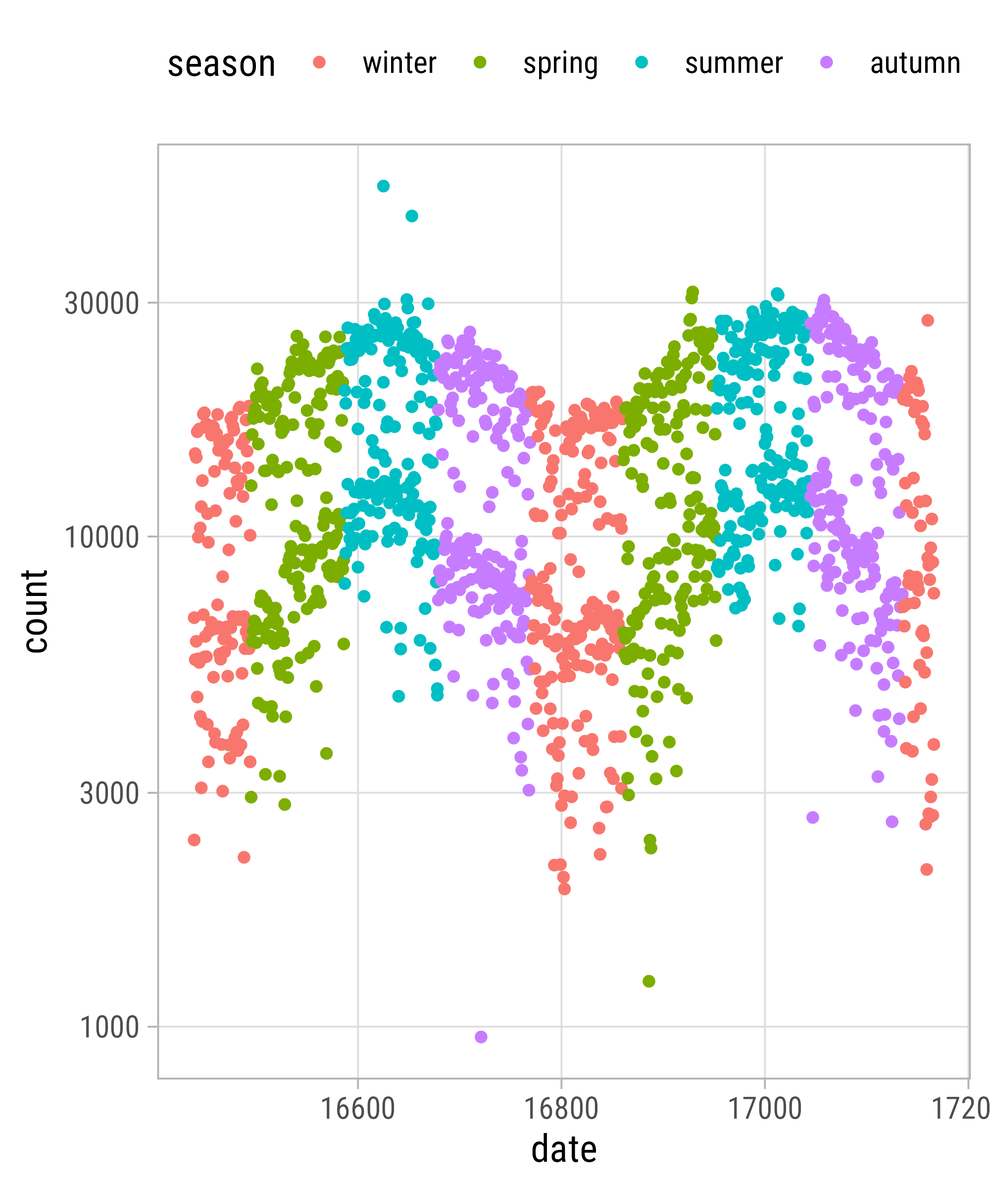
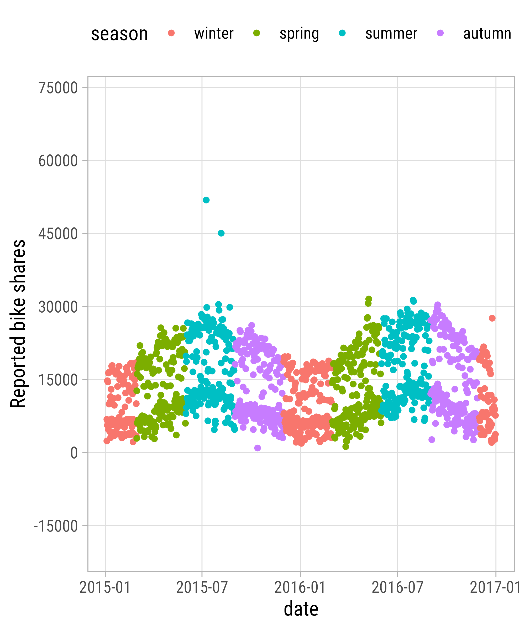
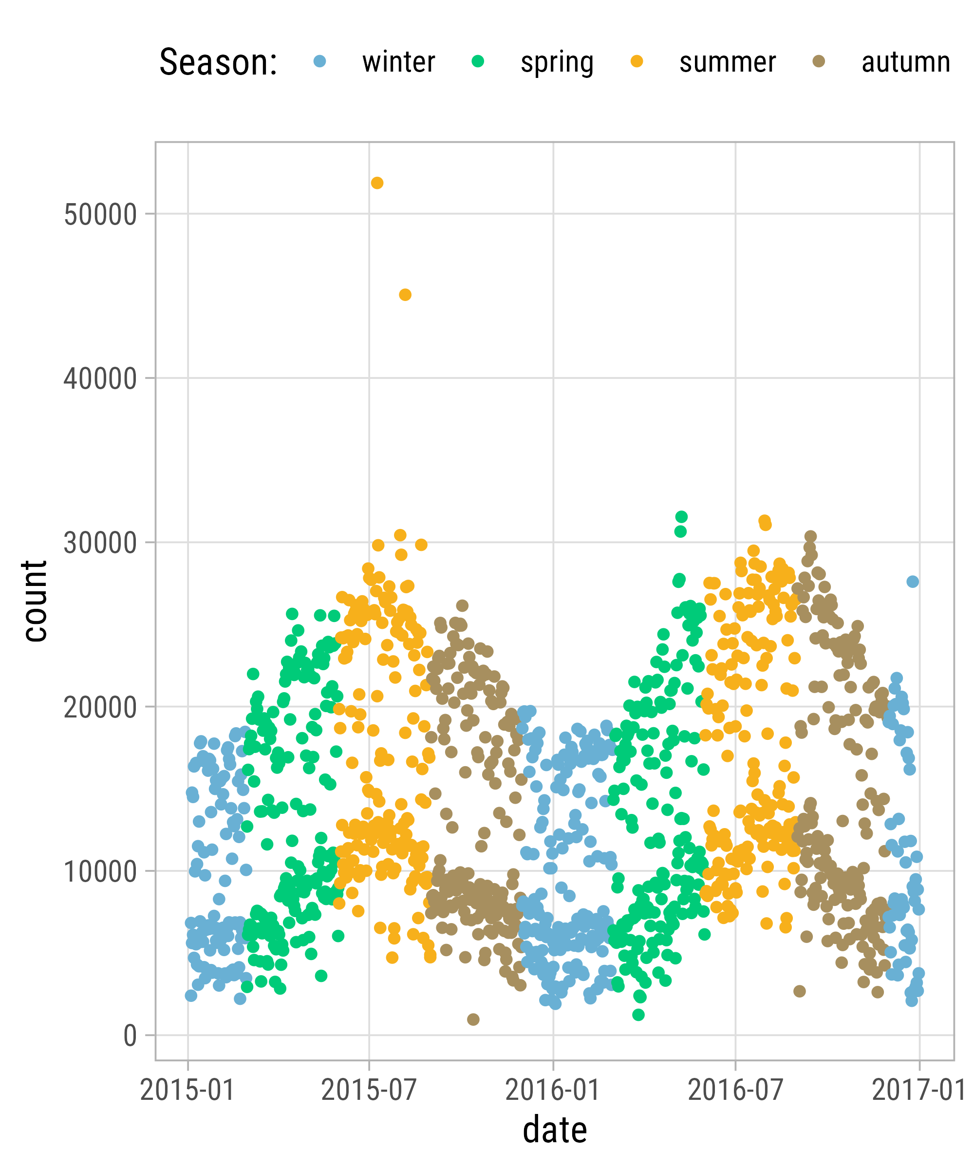
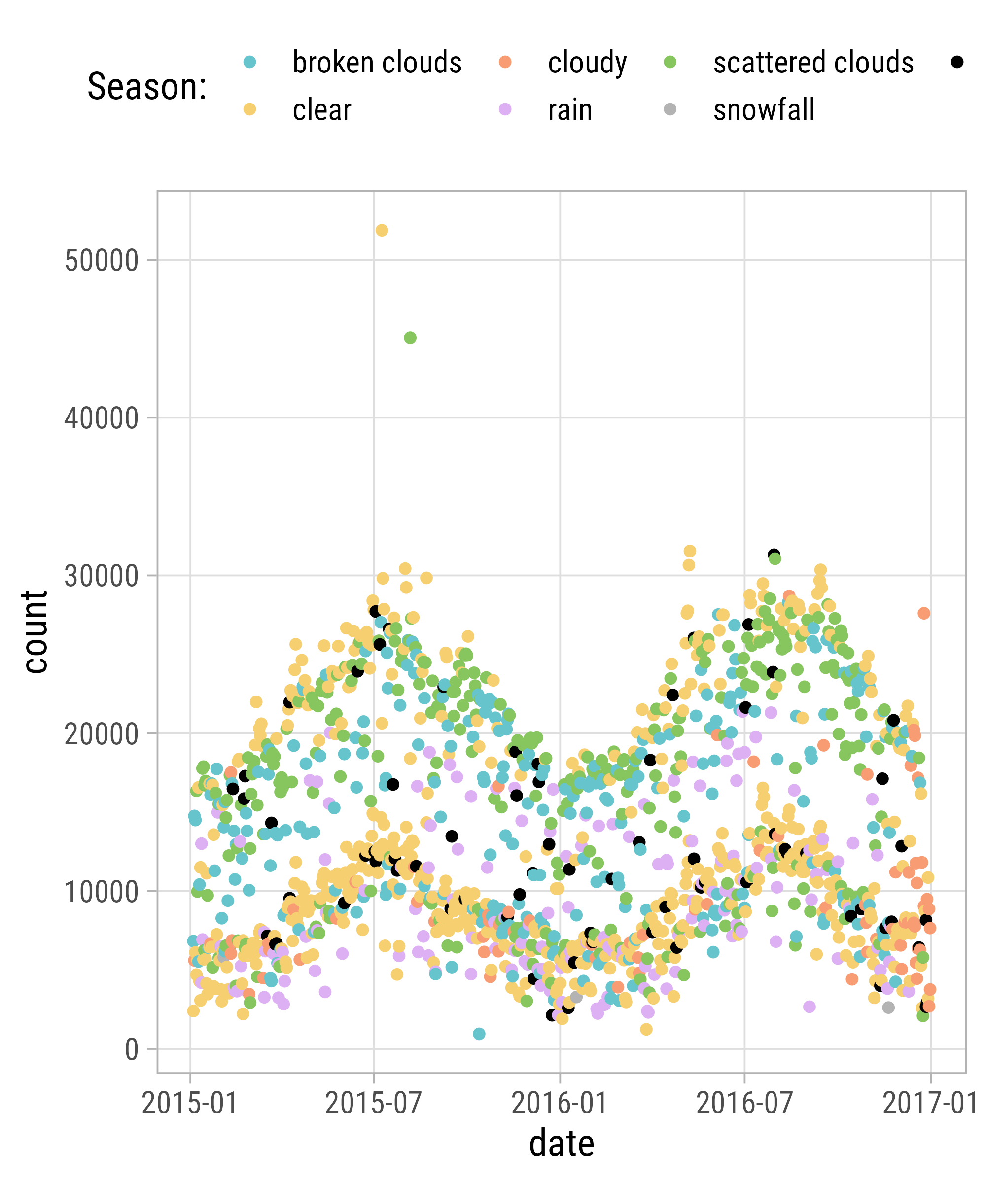
`scale_x|y_date`
`scale_x|y_date`
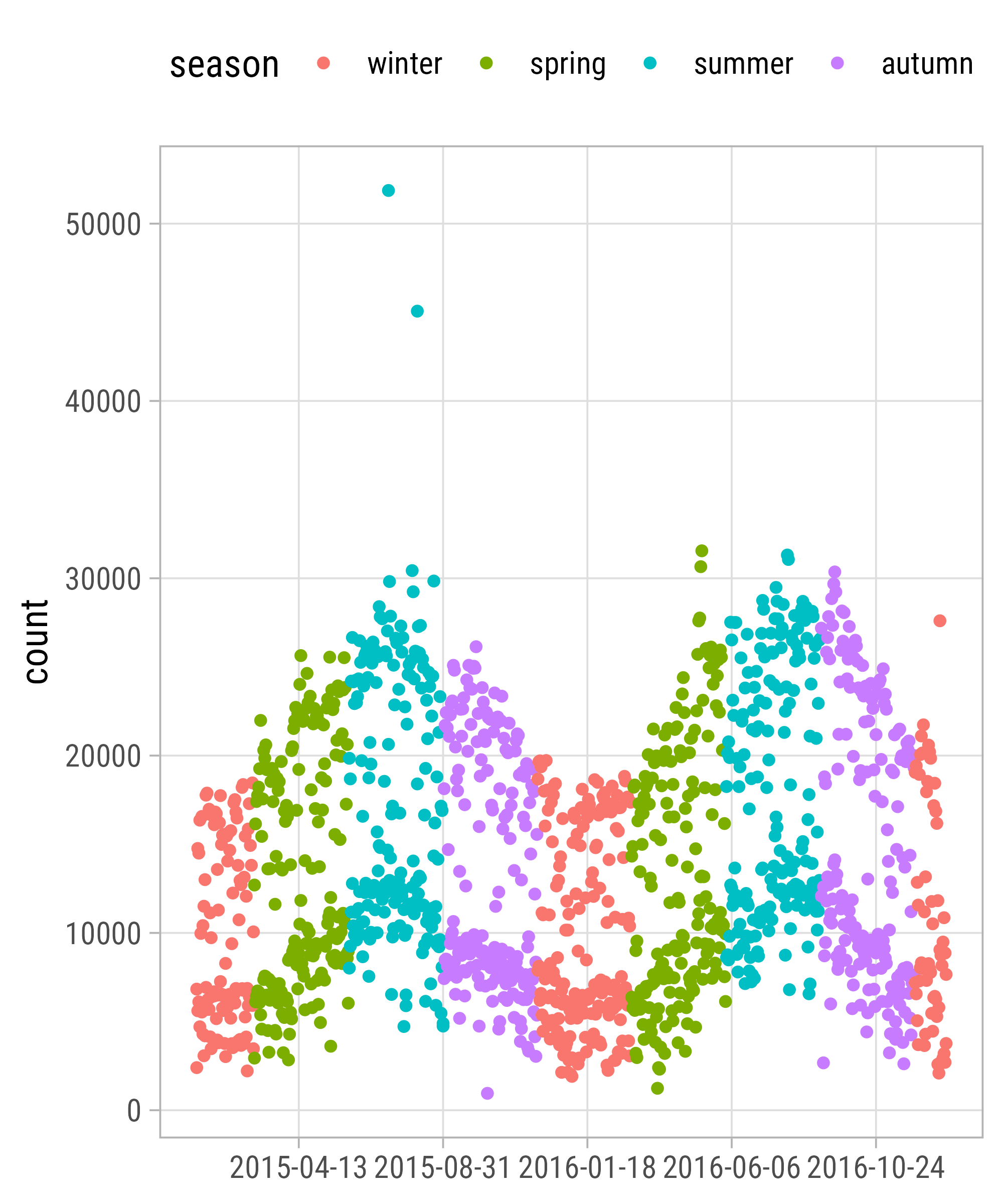
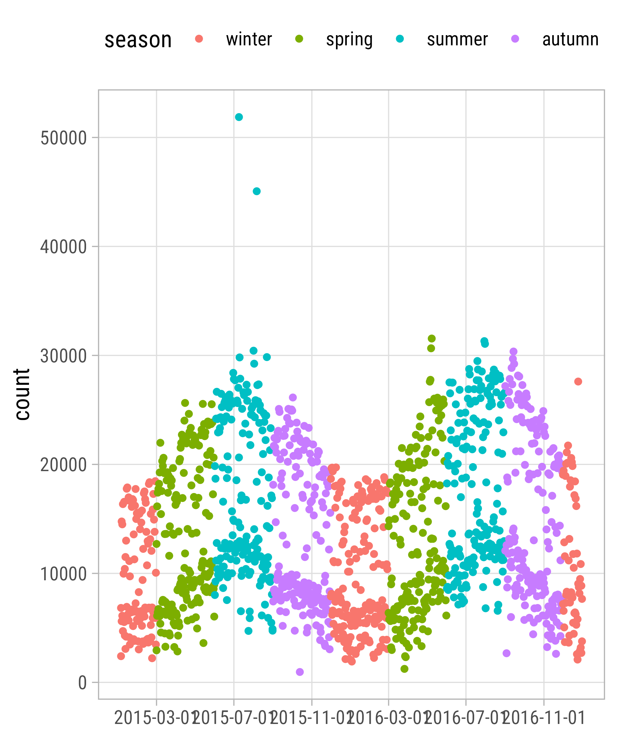
`scale_x|y_date` with `strftime()`

`scale_x|y_date` with `strftime()`

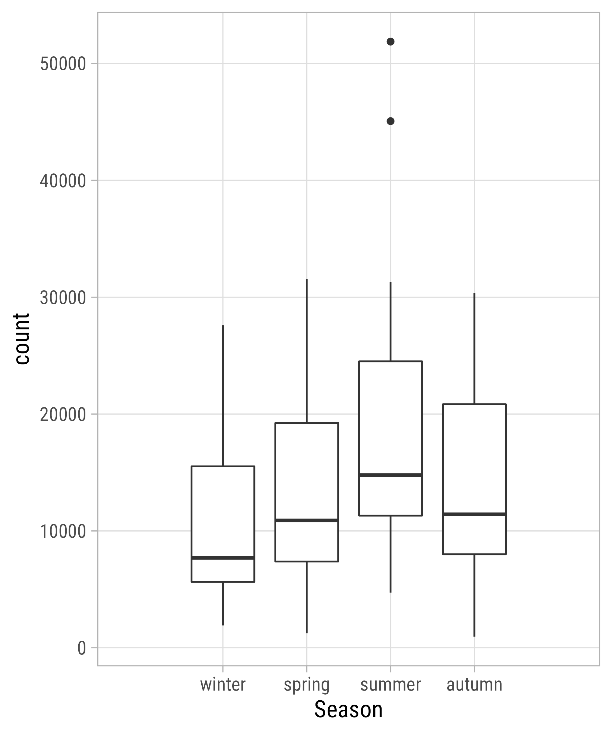
`scale_x|y_discrete`
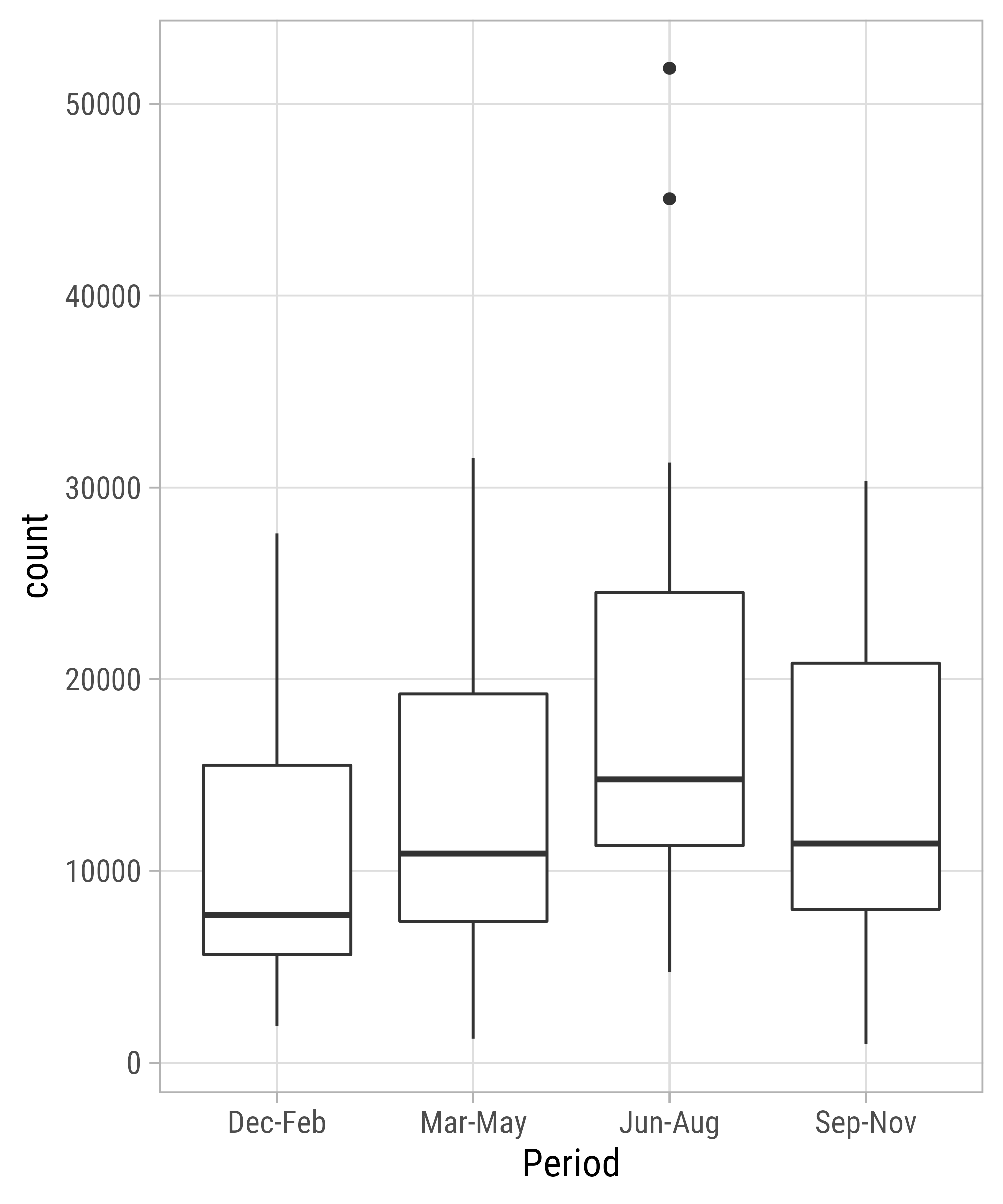
`scale_x|y_discrete`
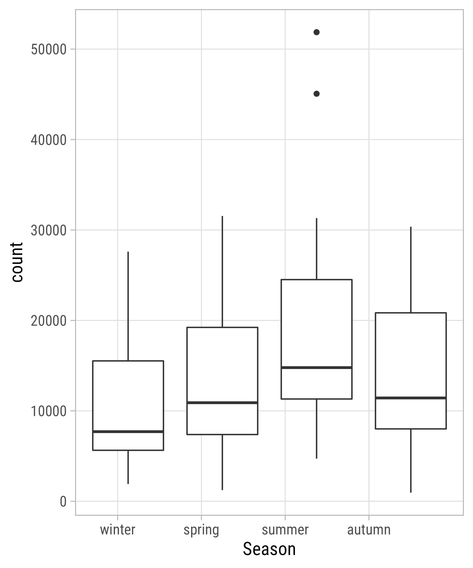
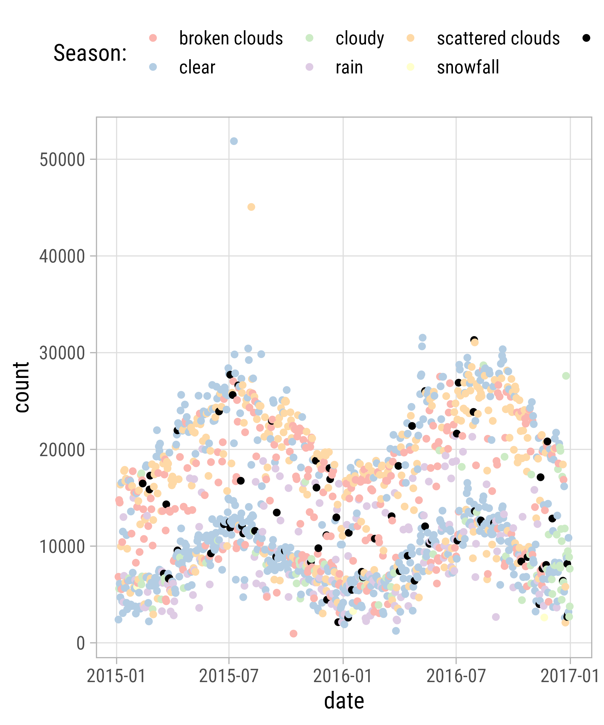
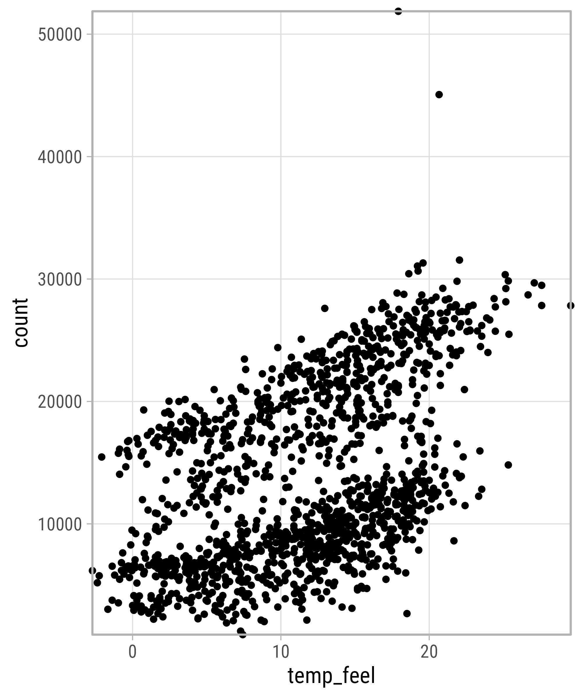
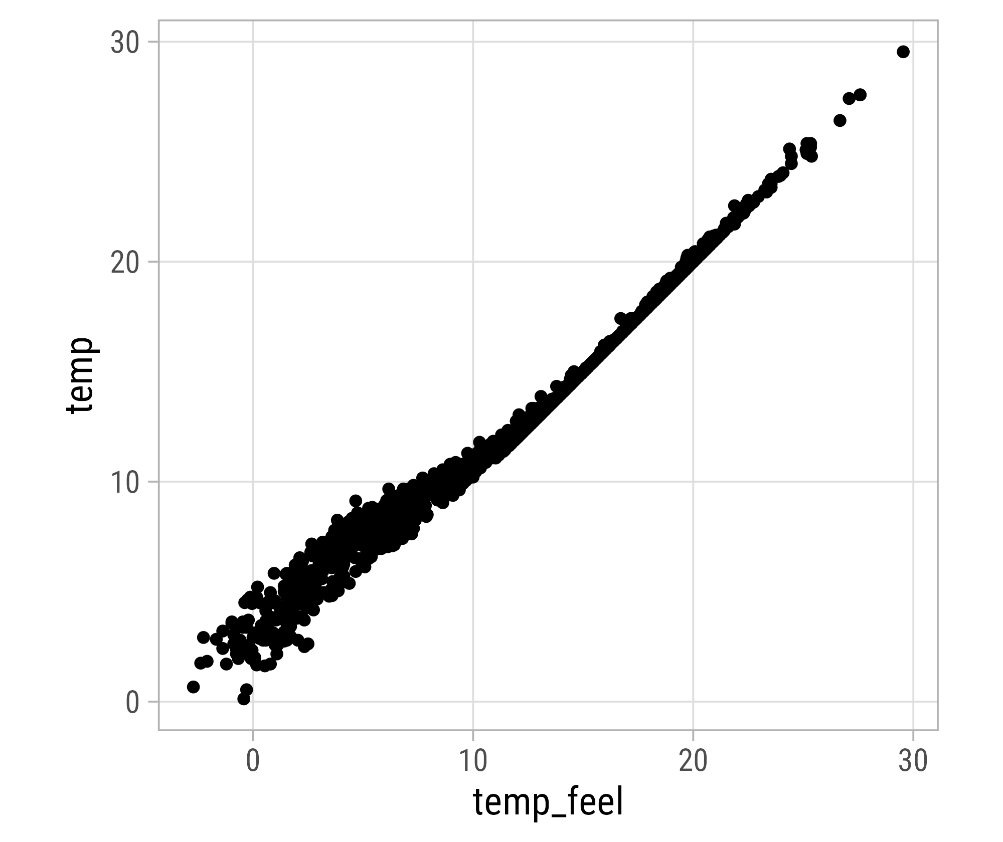
Discrete or Continuous?
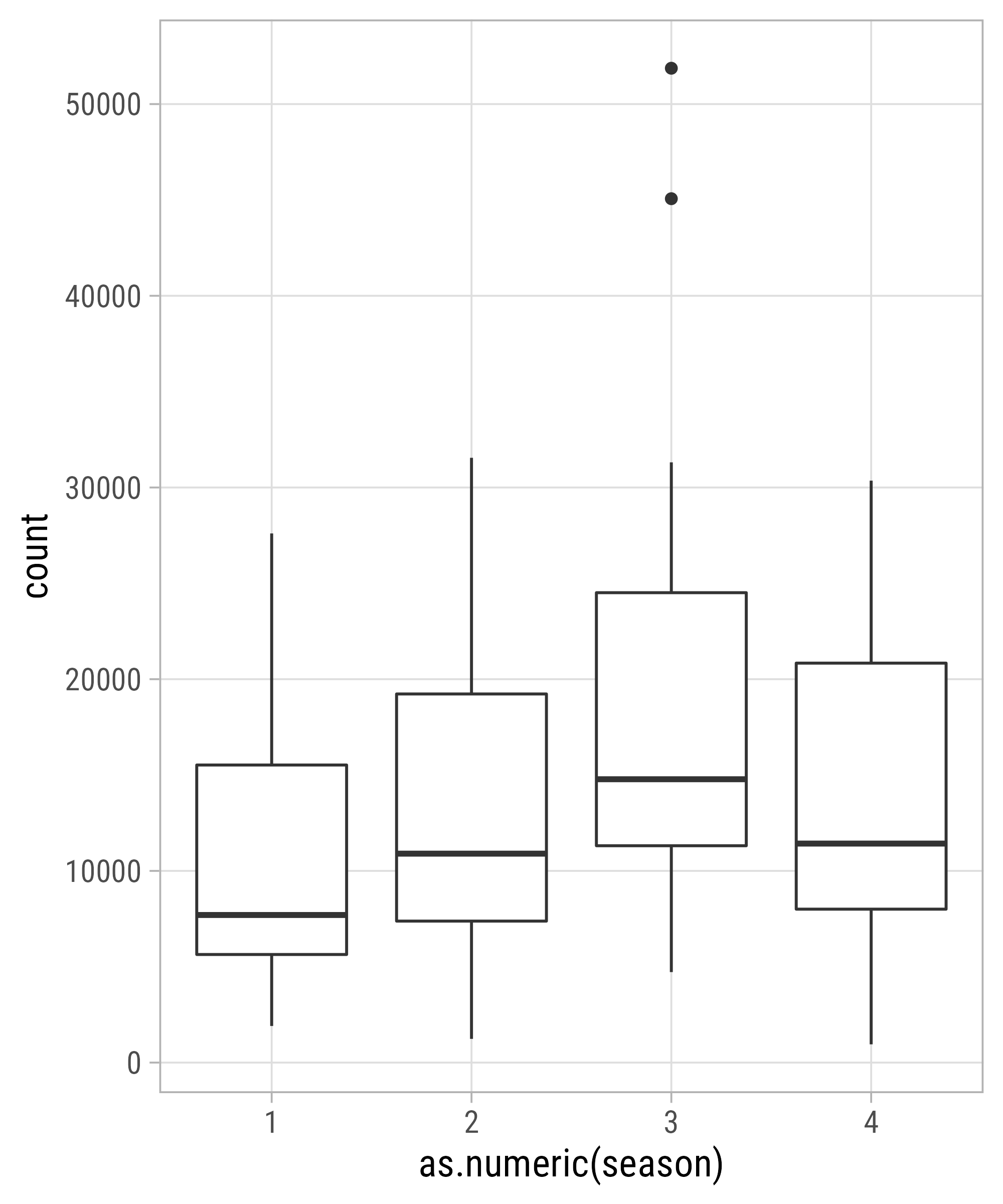
Discrete or Continuous?

Discrete or Continuous?
`scale_color|fill_discrete`
`scale_color|fill_discrete`

`scale_color|fill_discrete`
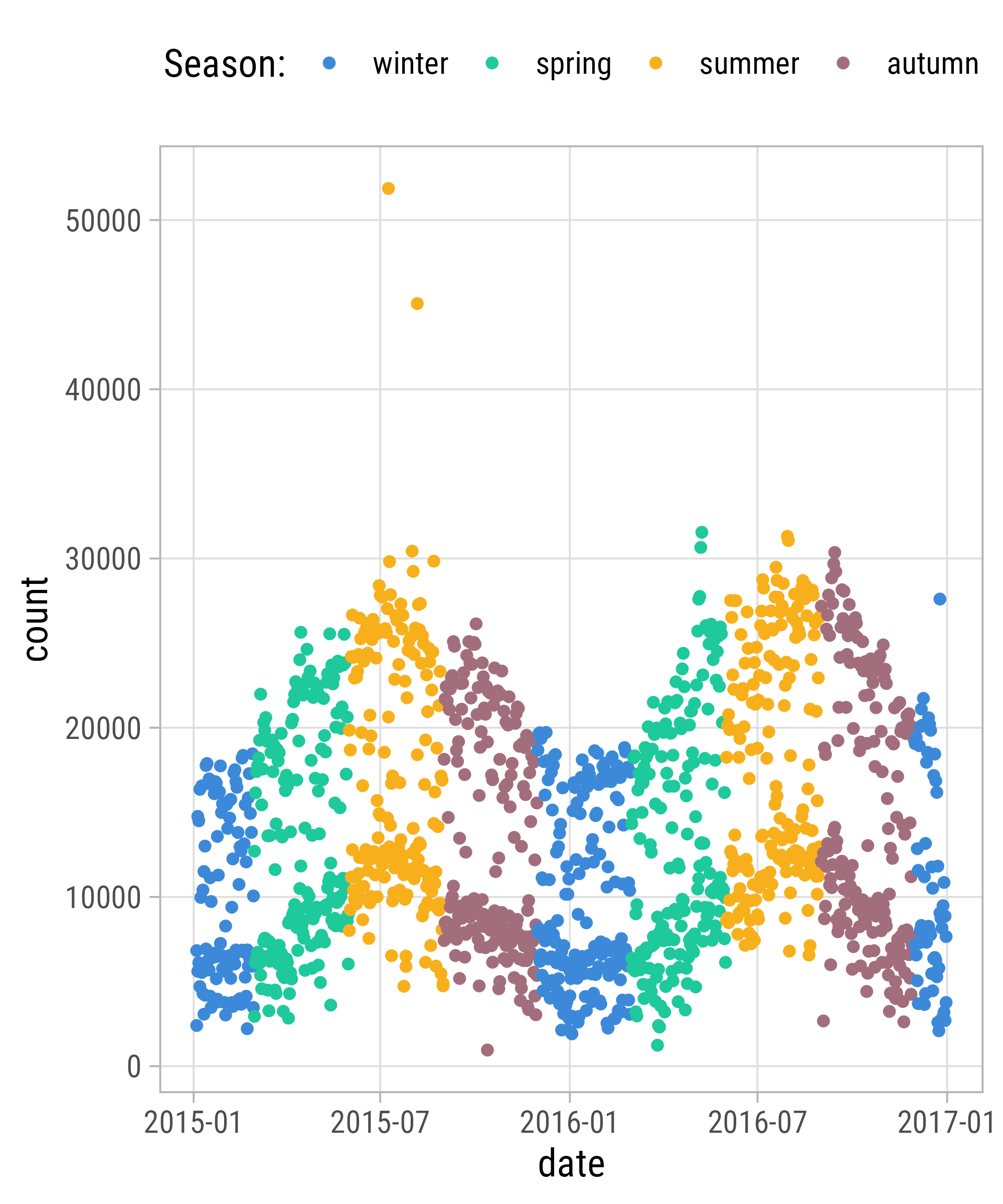
`scale_color|fill_discrete`
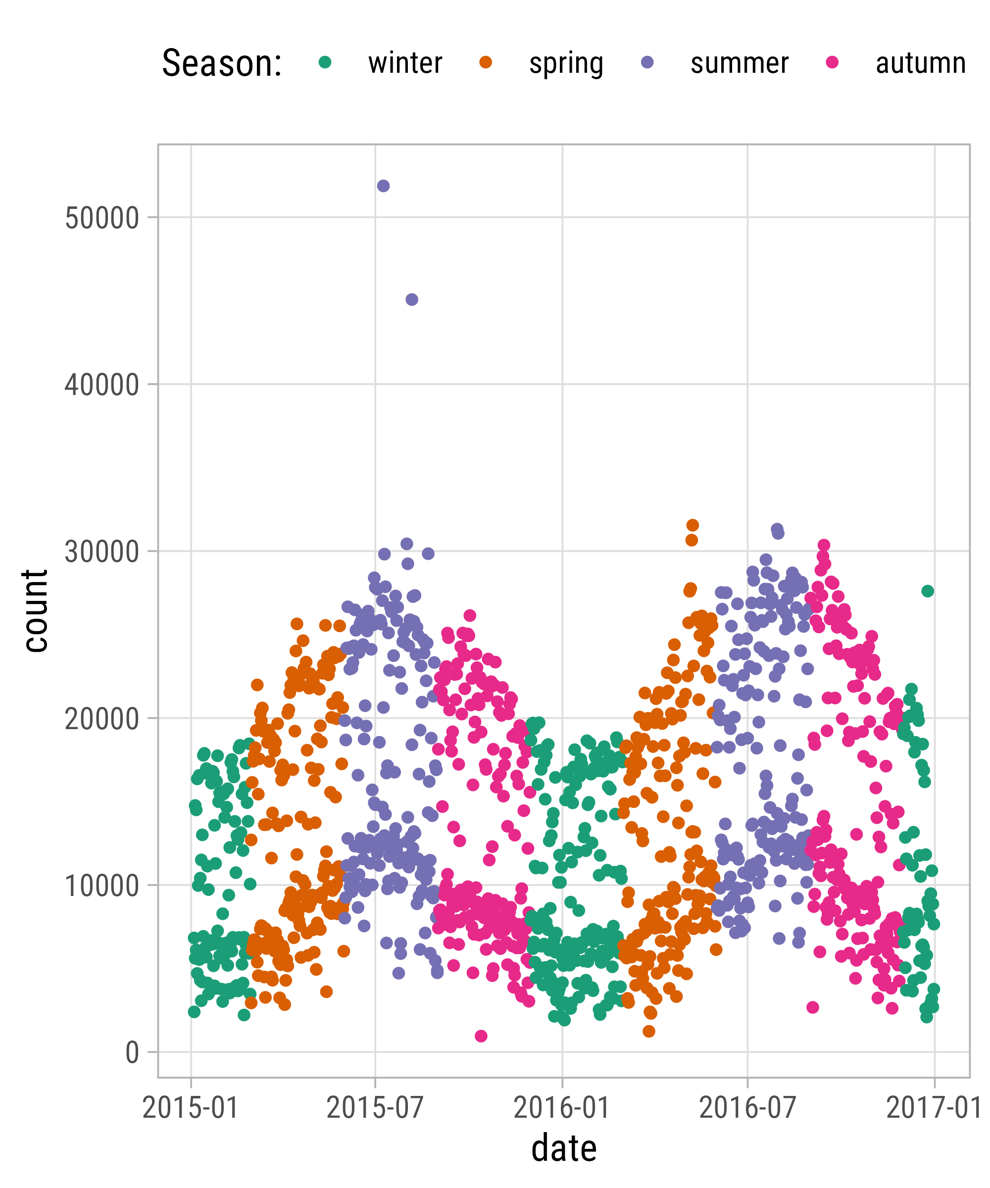
`scale_color|fill_manual`
`scale_color|fill_carto_d`
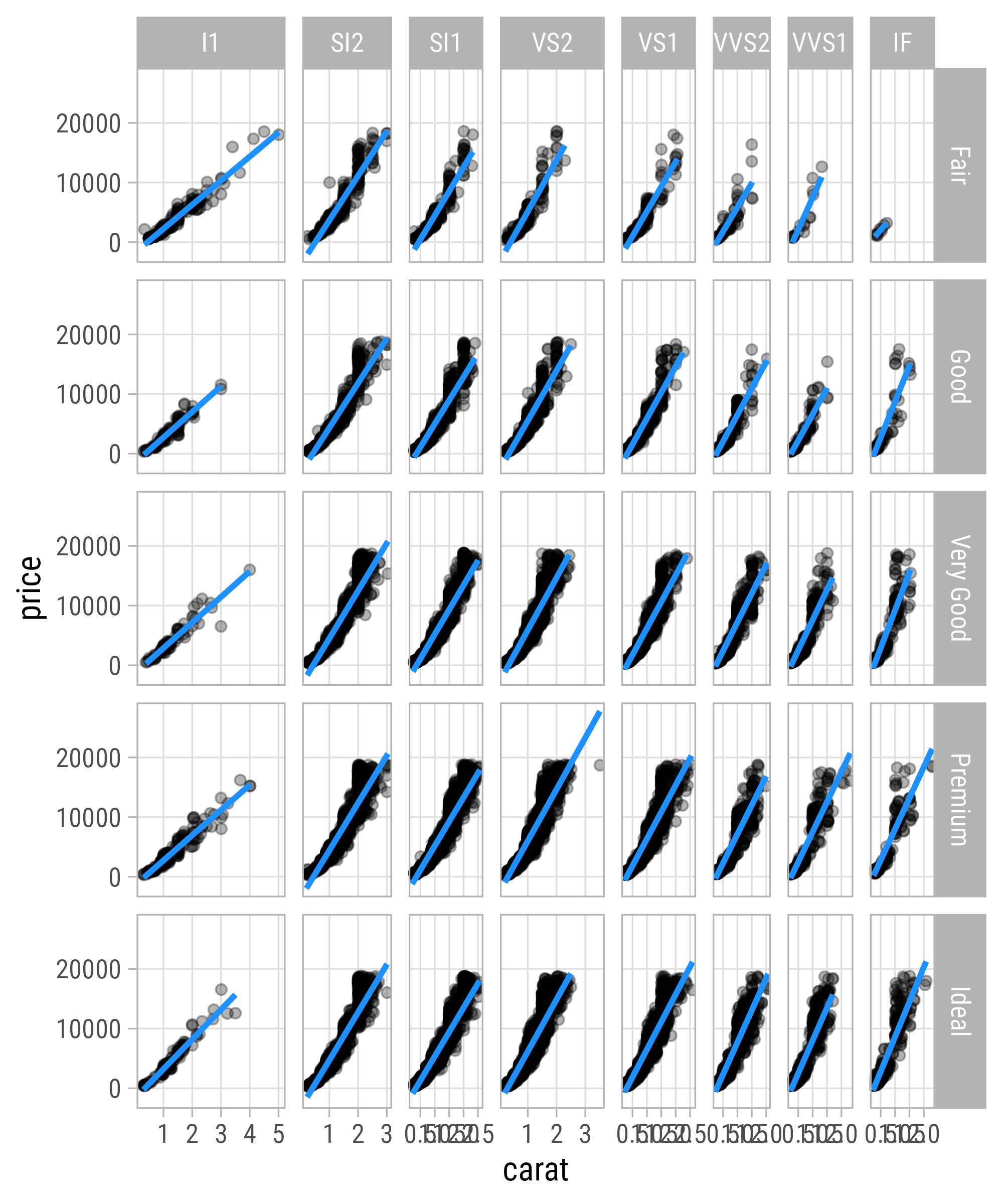
Your Turn!
Modify our diamonds facet like this:
Diamonds Facet
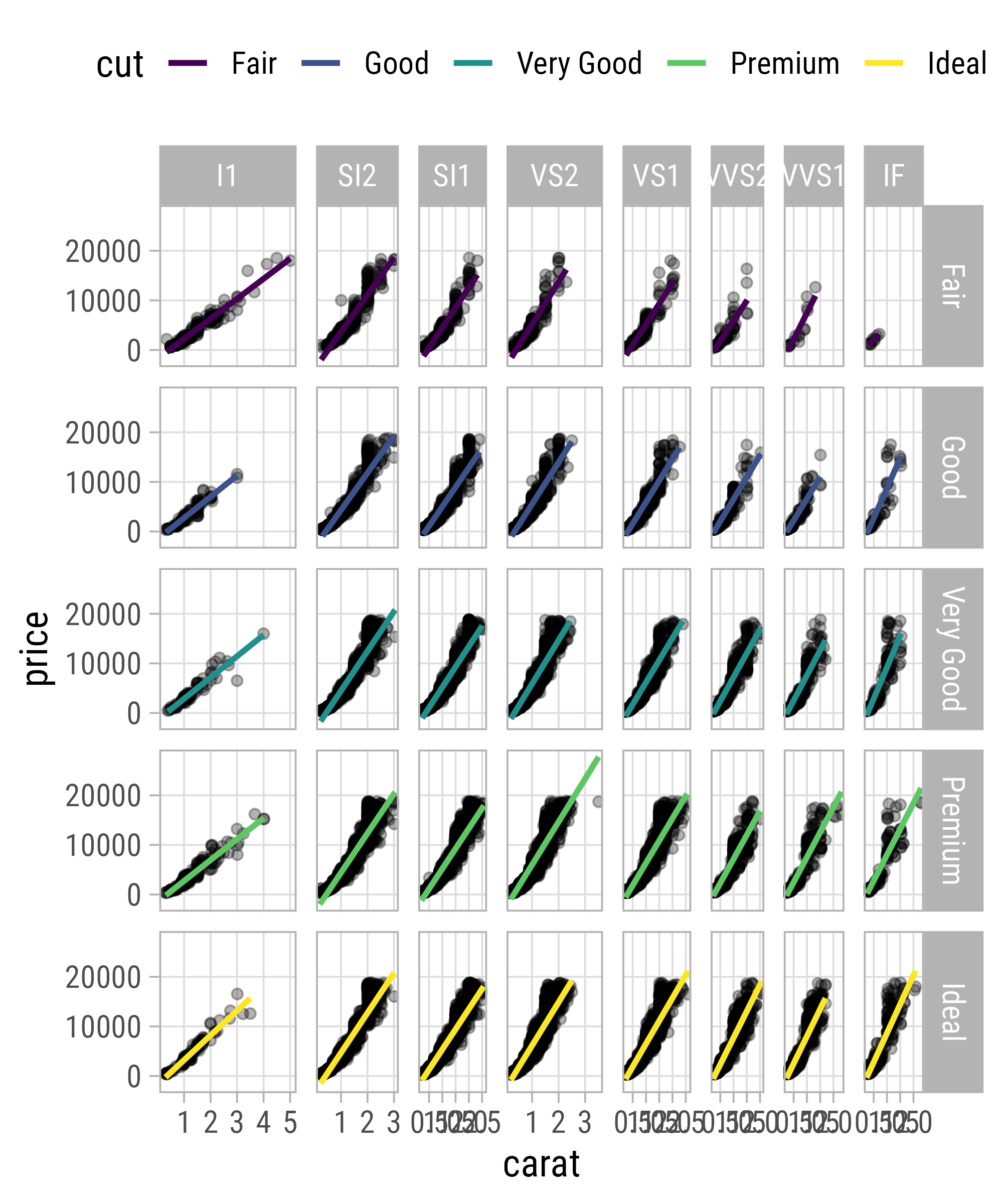
Diamonds Facet

Diamonds Facet
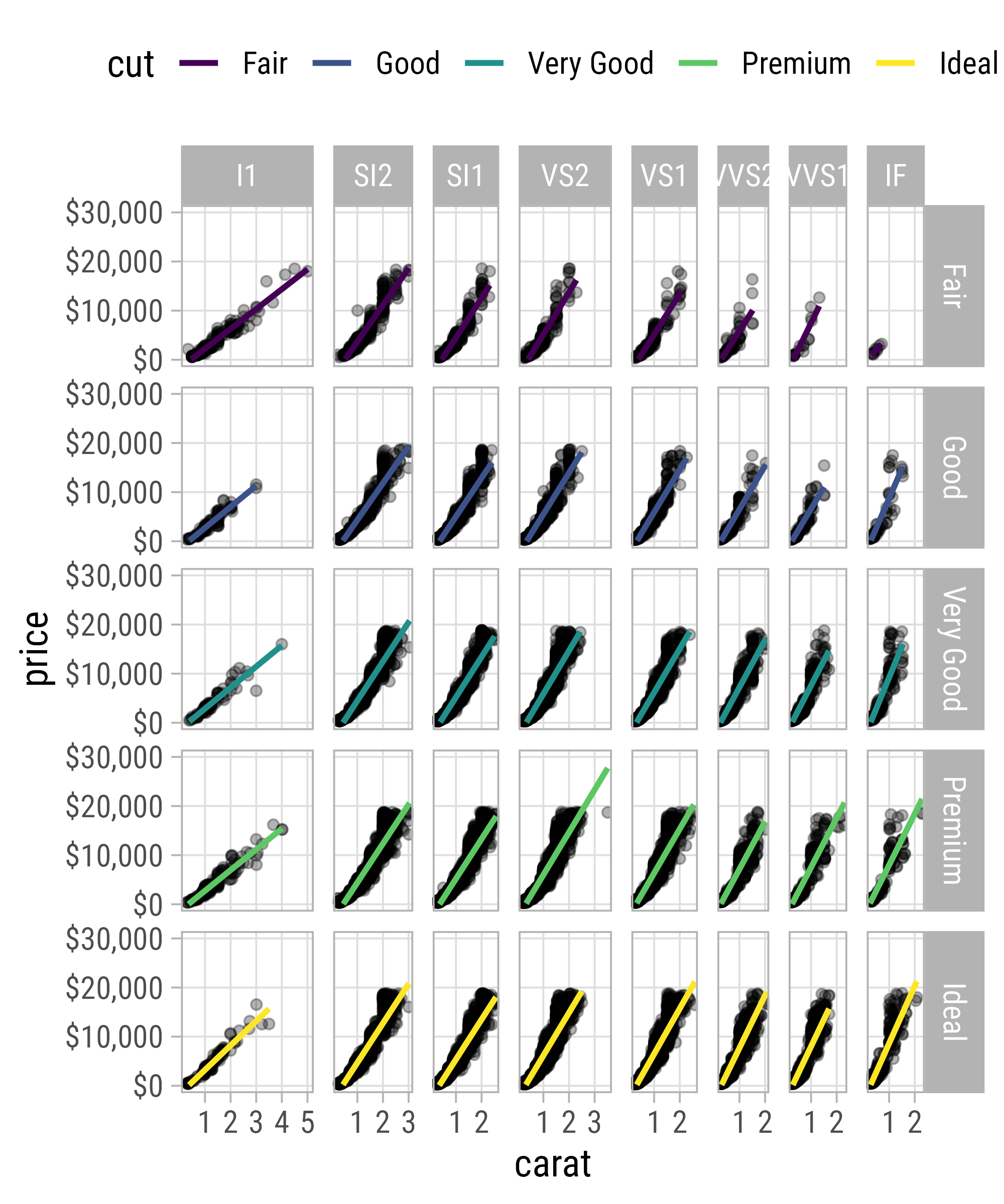
Diamonds Facet

Diamonds Facet

Diamonds Facet

Diamonds Facet
Cartesian Coordinate System
Cartesian Coordinate System
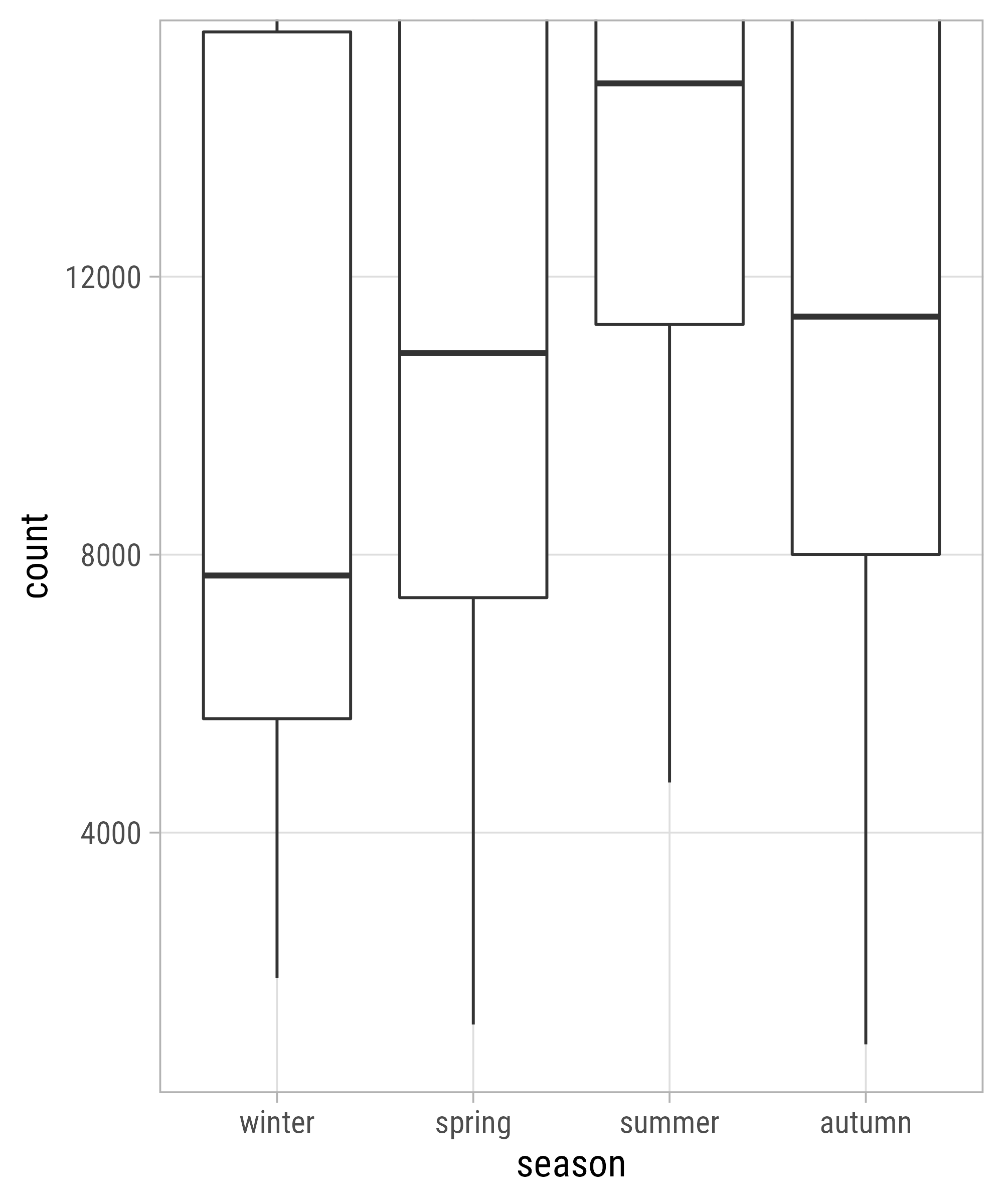
Changing Limits
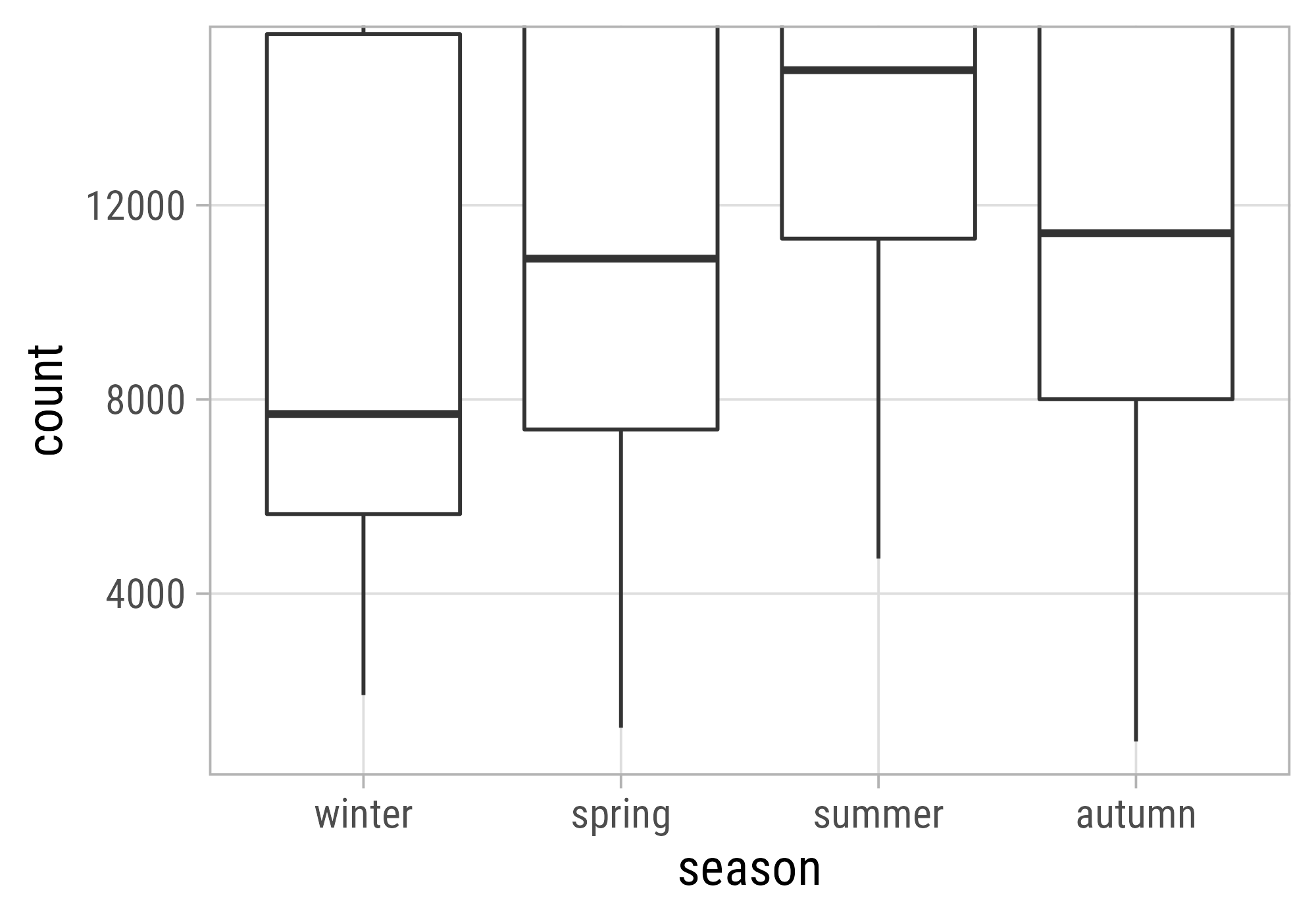
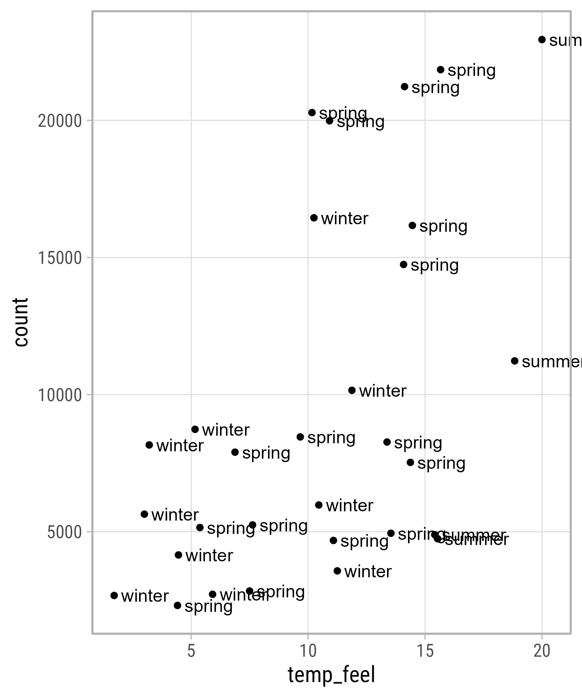
Clipping
Clipping
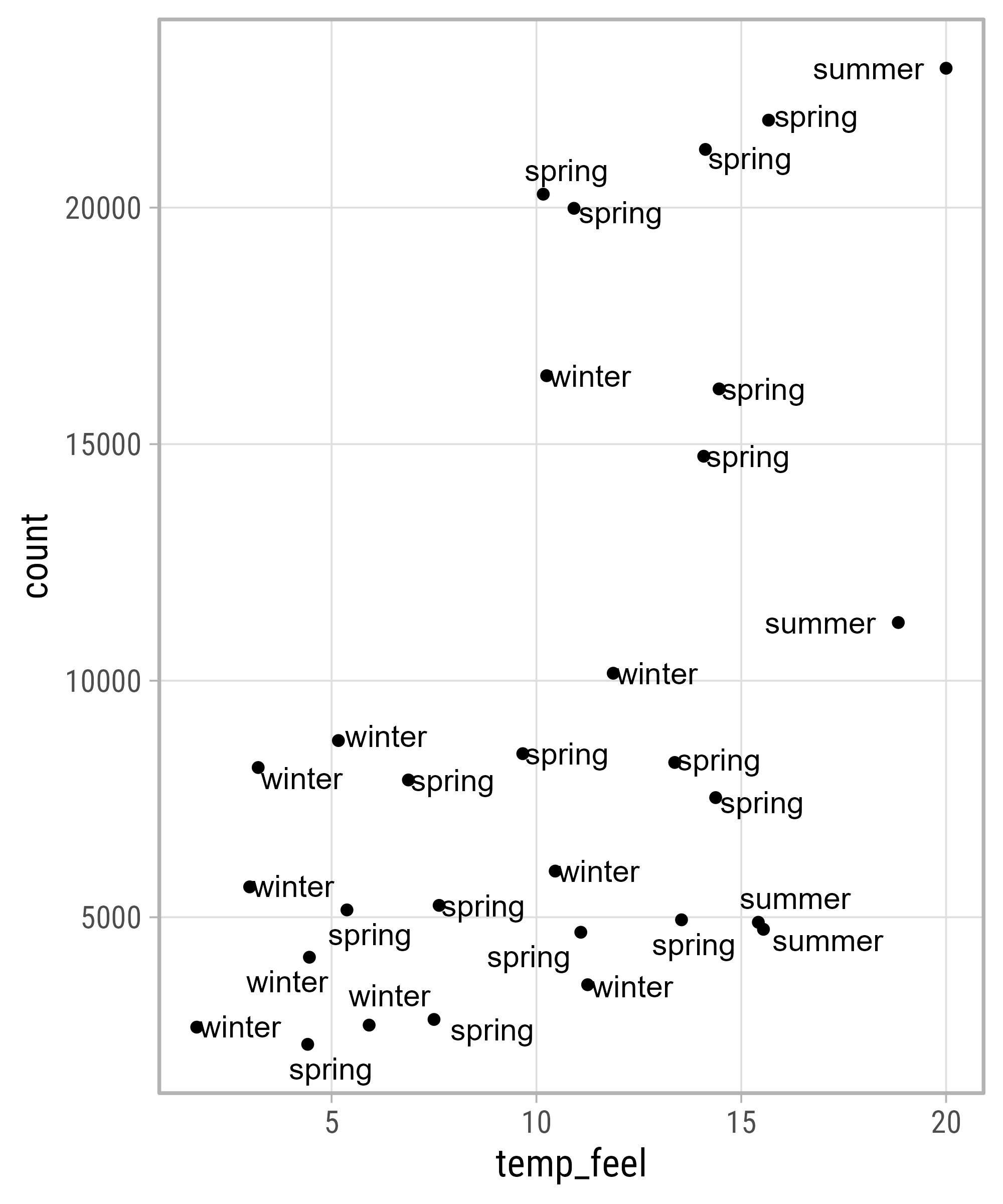
… or better use {ggrepel}
Remove All Padding
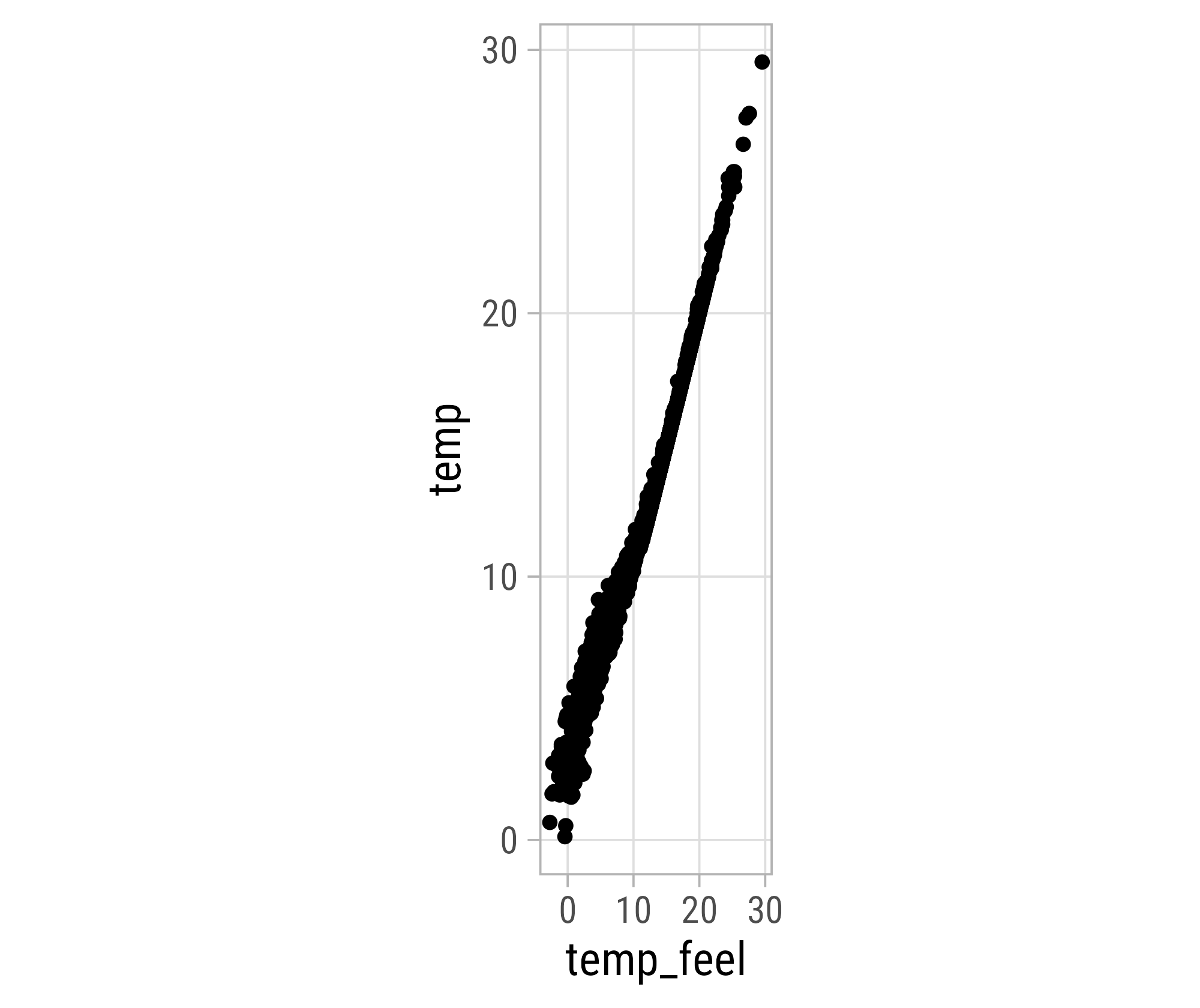
Fixed Coordinate System
Flipped Coordinate System
Flipped Coordinate System


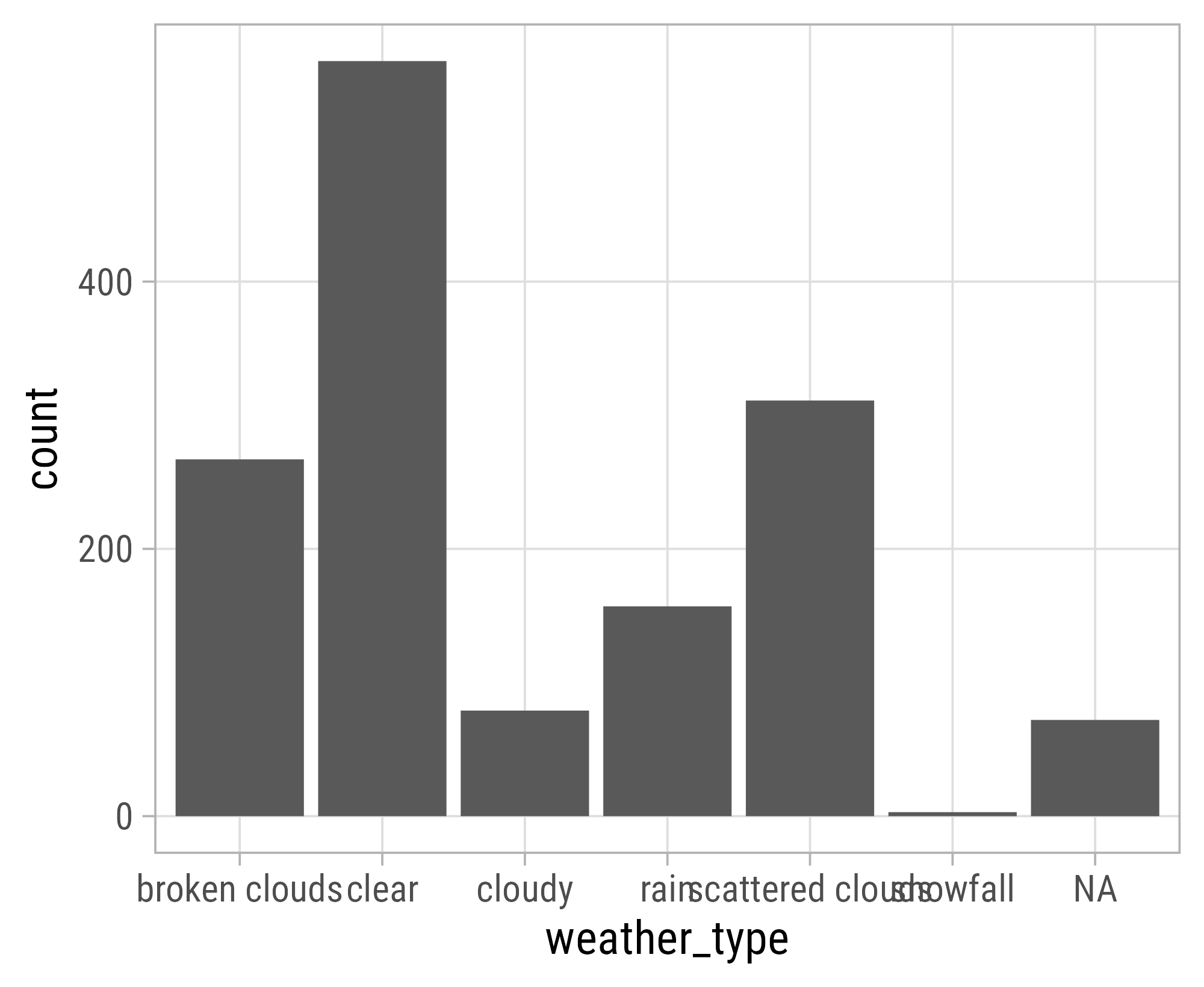
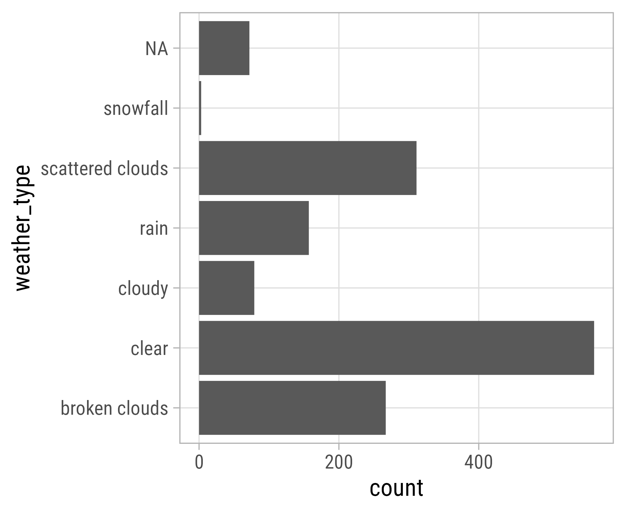
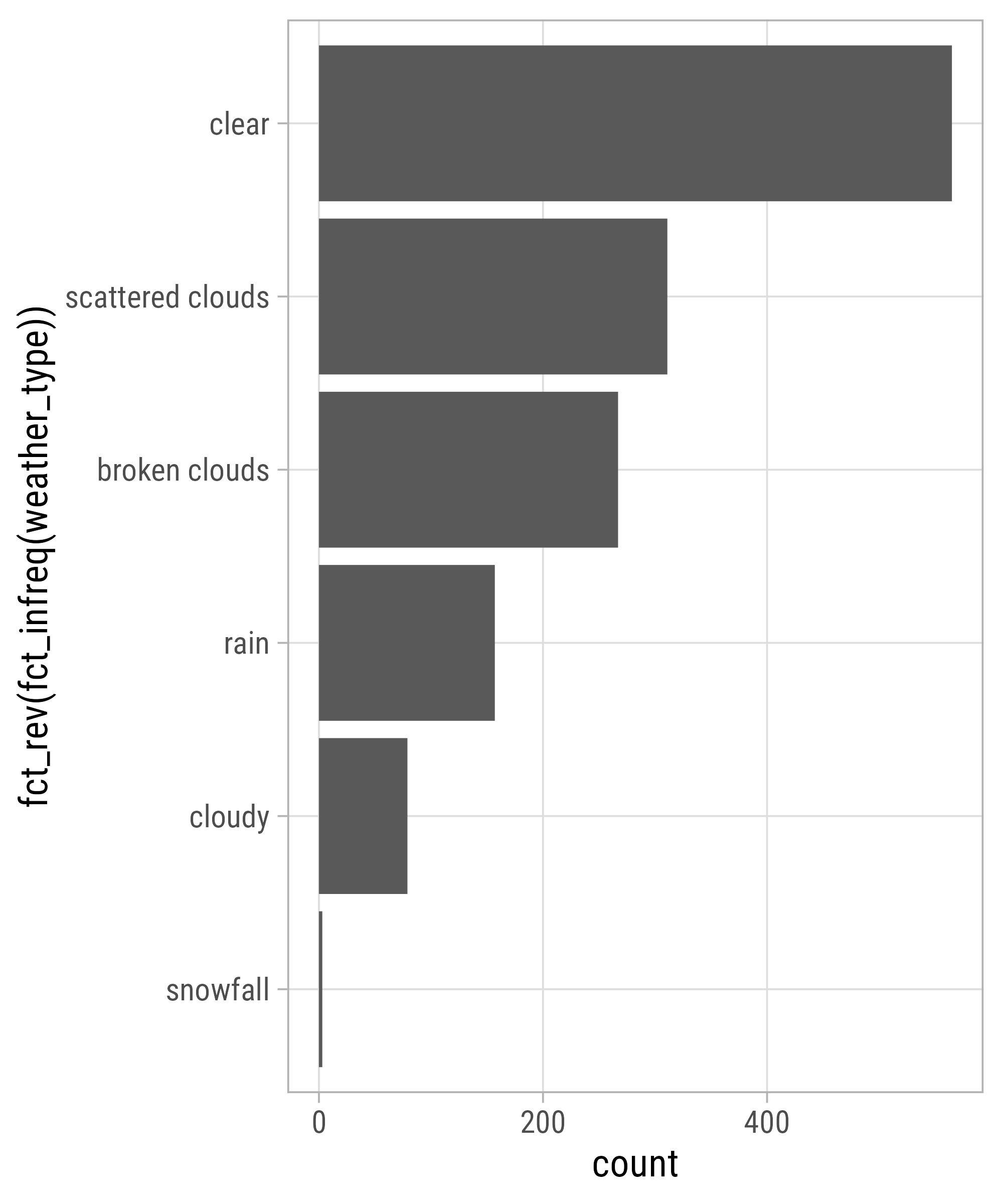
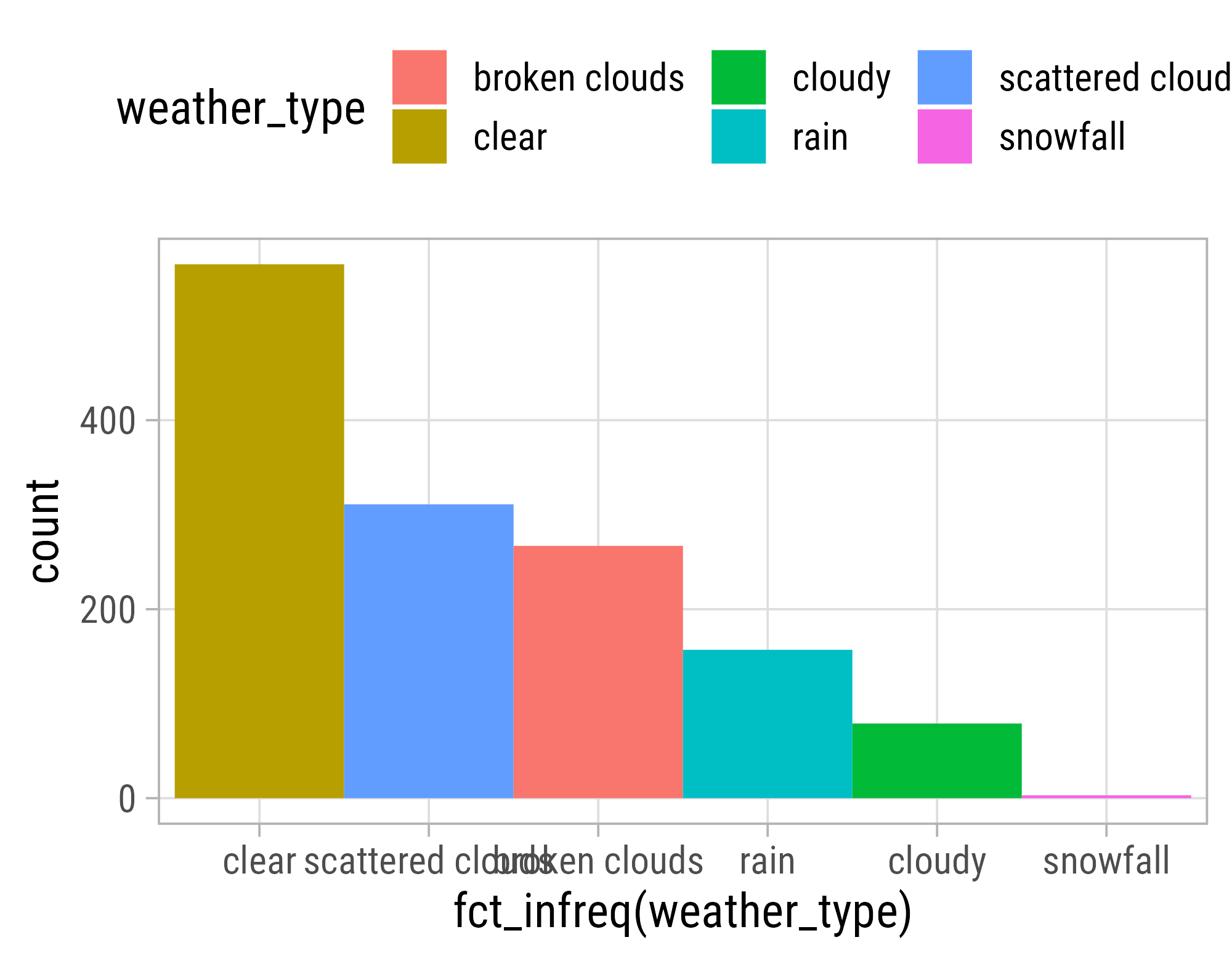
Reminder: Sort Your Bars!
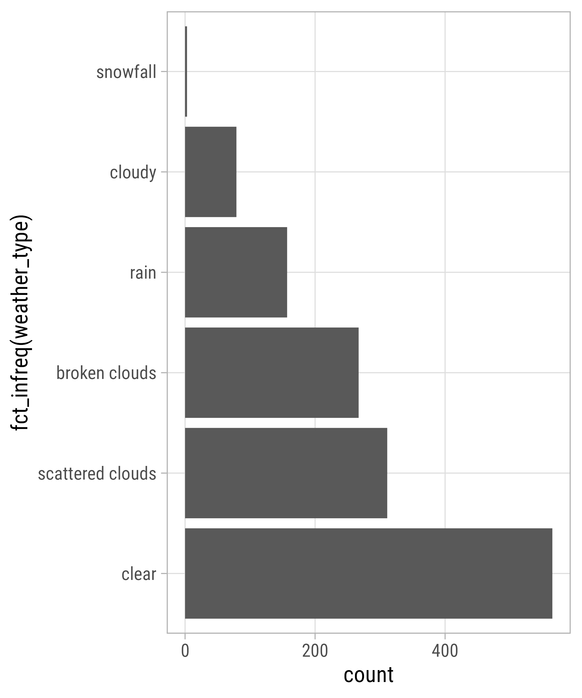
Reminder: Sort Your Bars!
Circular Corrdinate System

Circular Cordinate System

Circular Corrdinate System
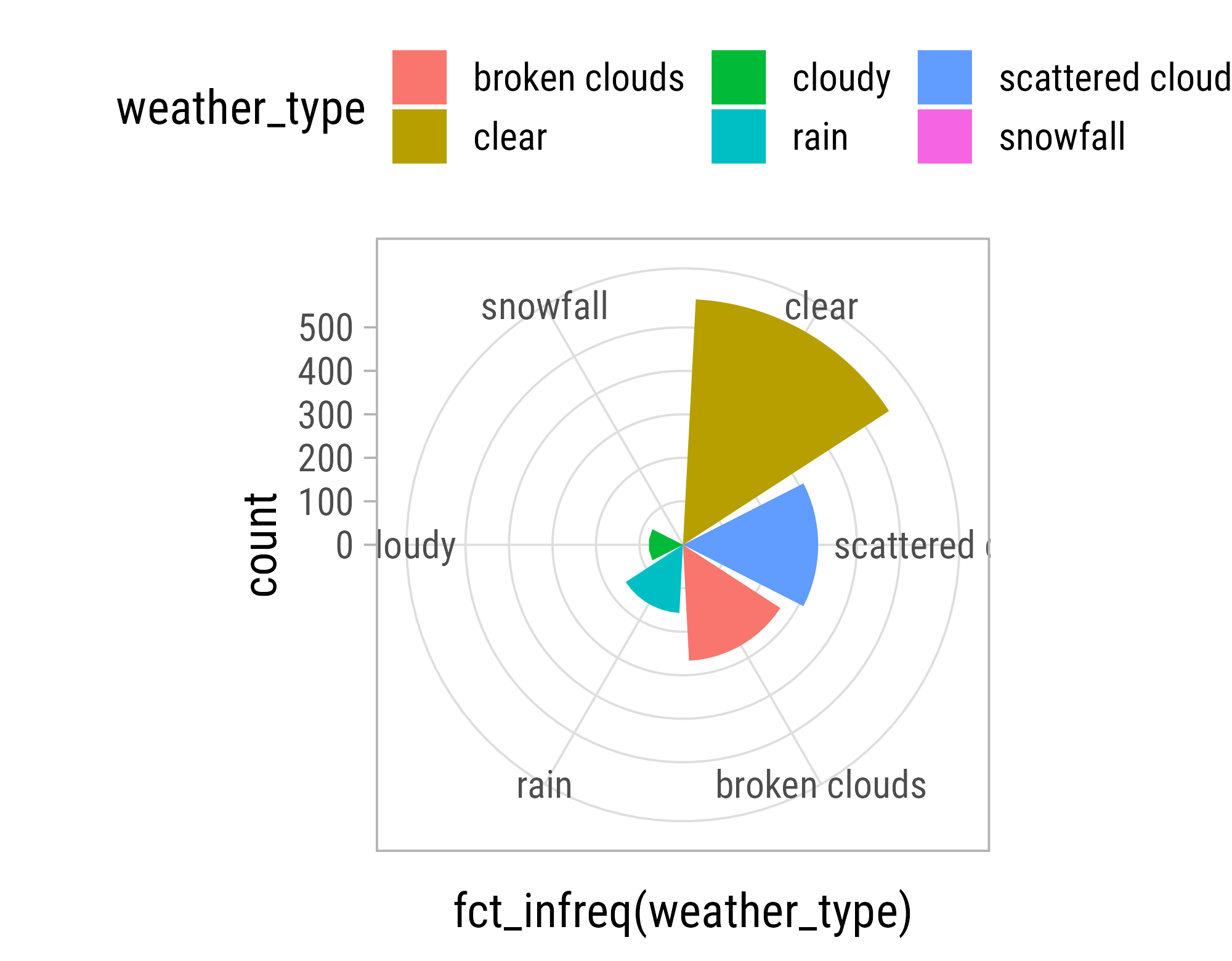
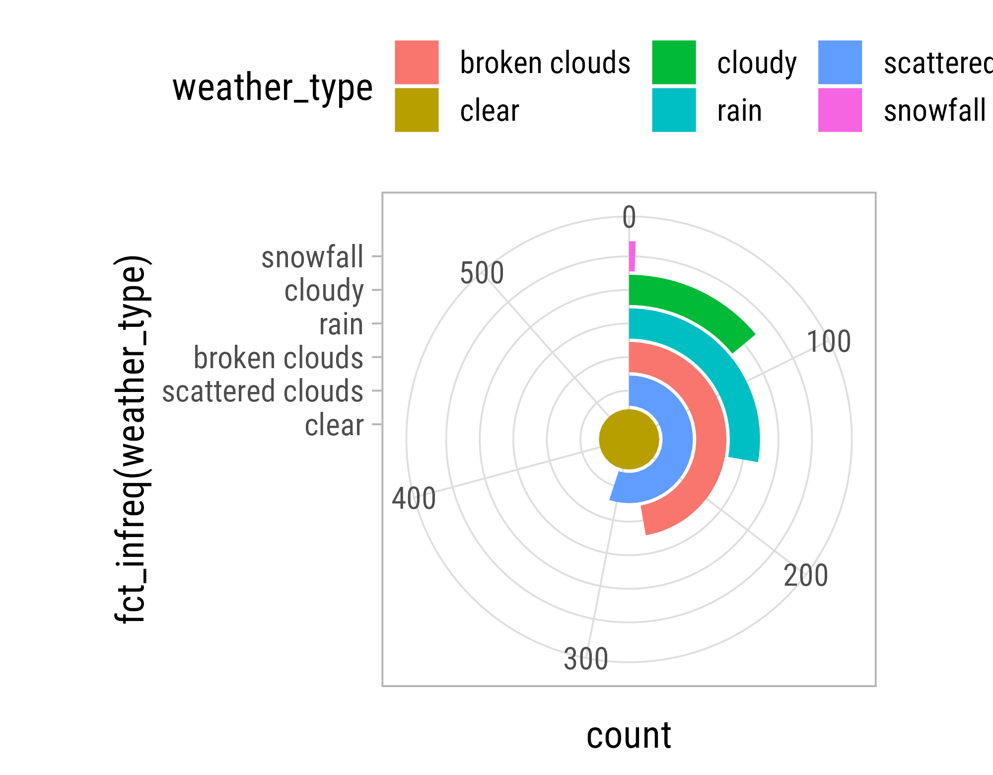
Circular Corrdinate System

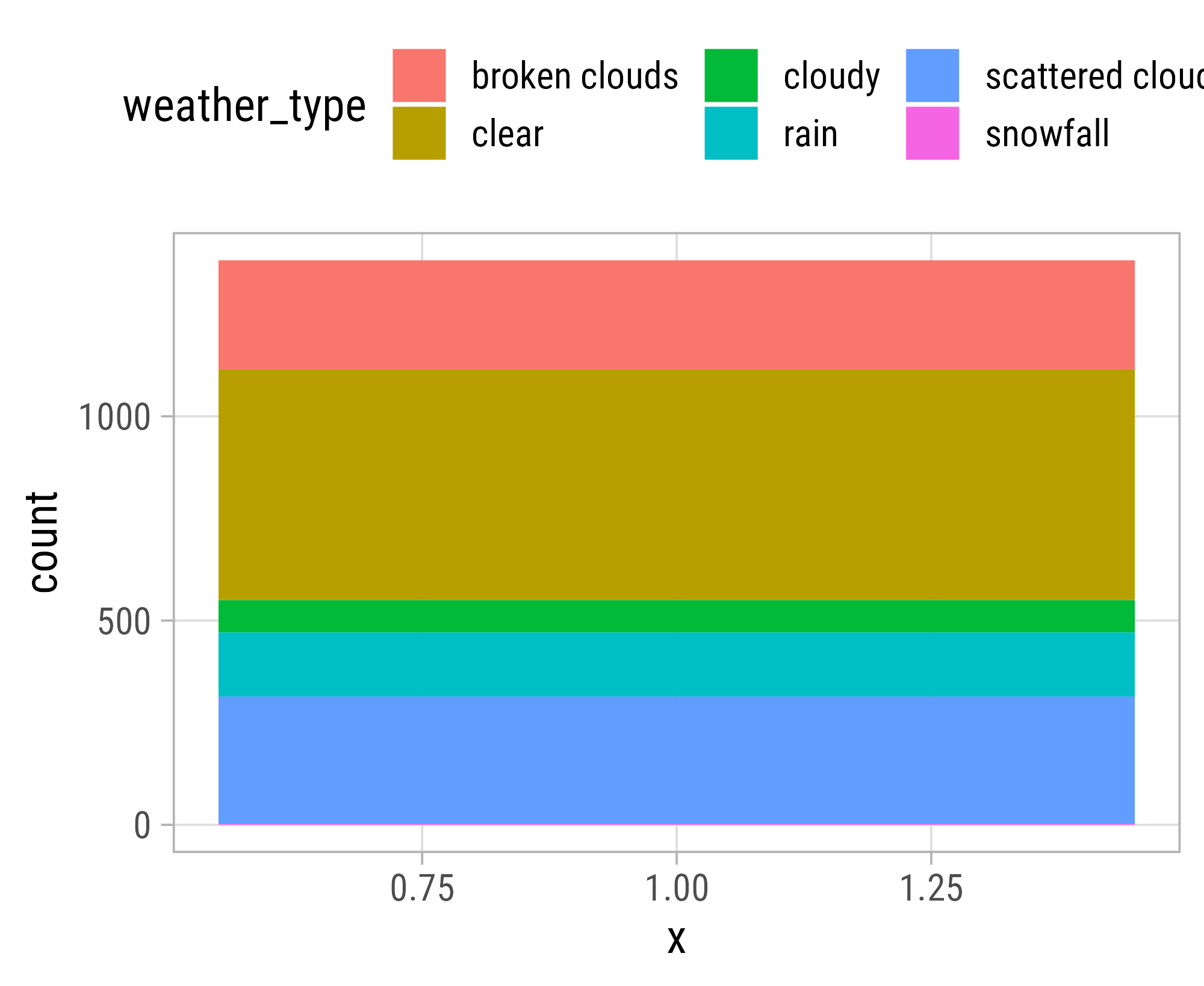
Circular Corrdinate System


Transform a Coordinate System
Transform a Coordinate System
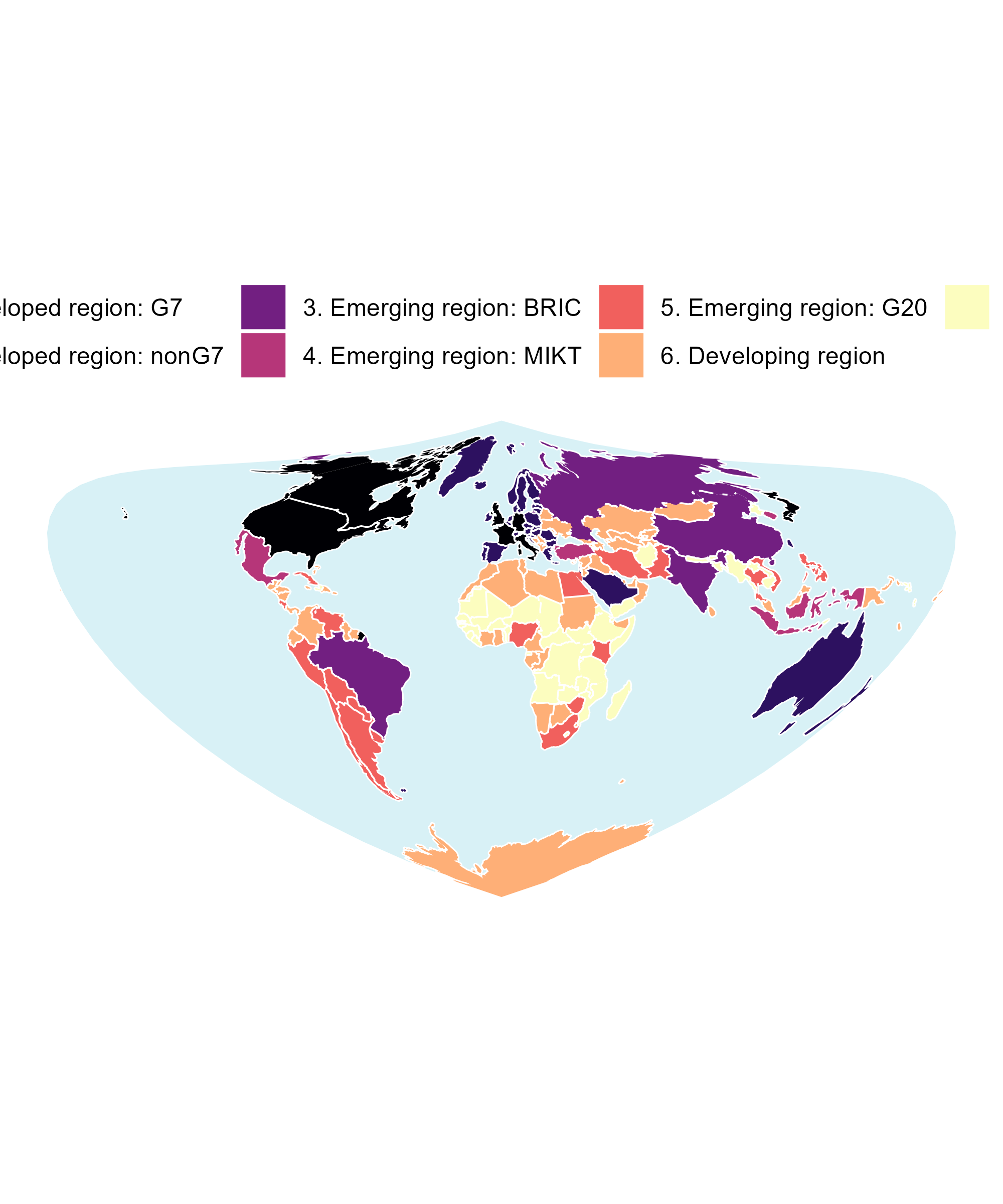
Spatial Coordinate (Reference) Systems
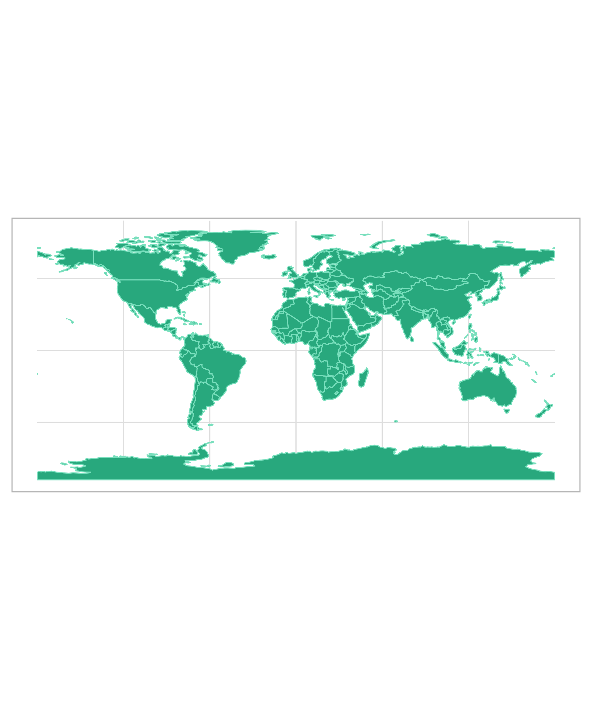
Spatial Coordinate (Reference) Systems
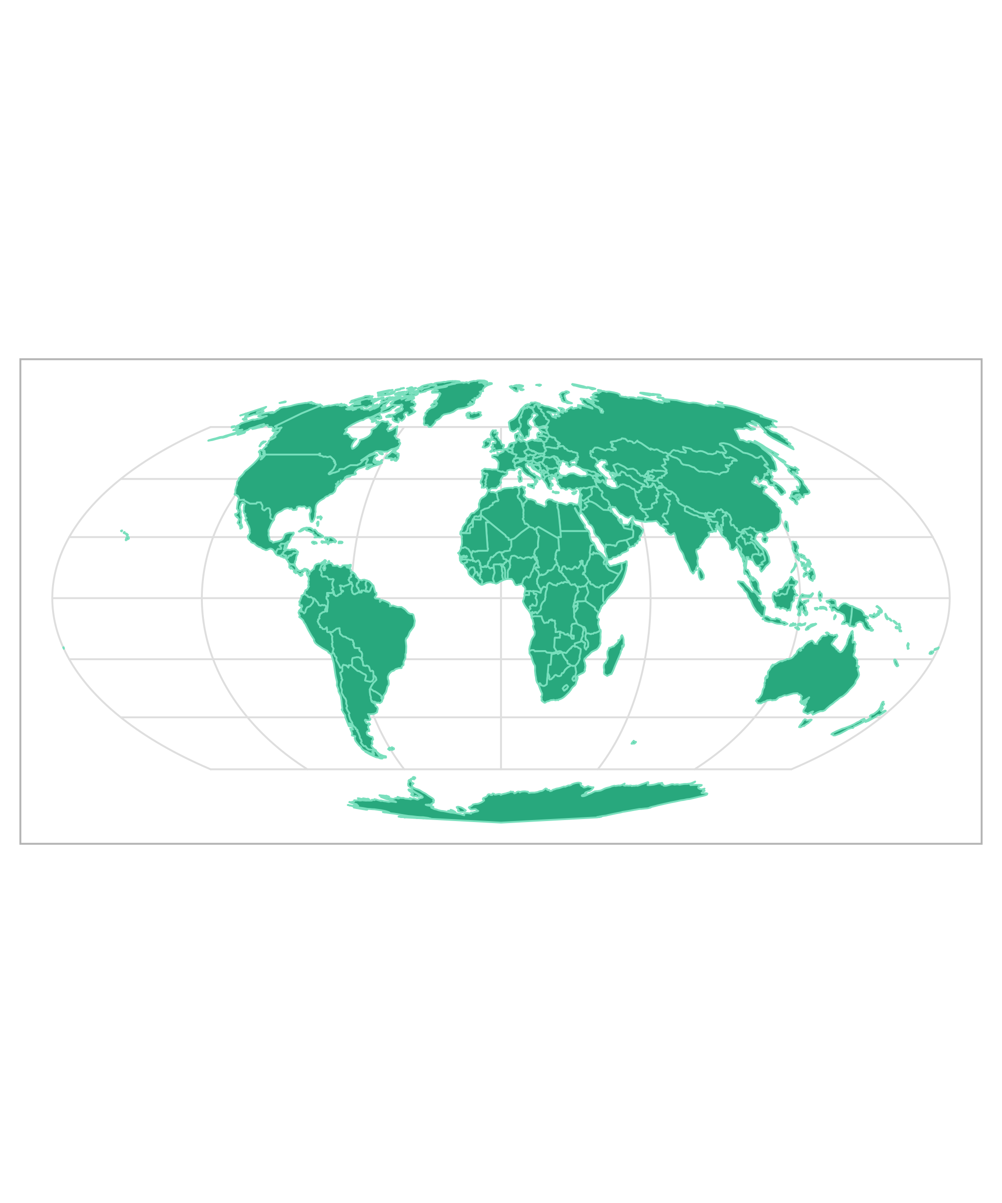
Spatial Coordinate (Reference) Systems
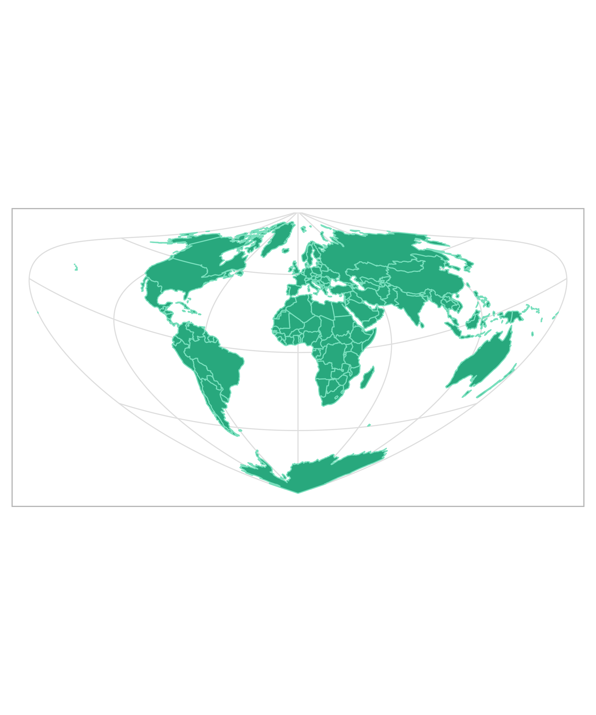
Spatial Coordinate (Reference) Systems
Mapping of Visual Properties
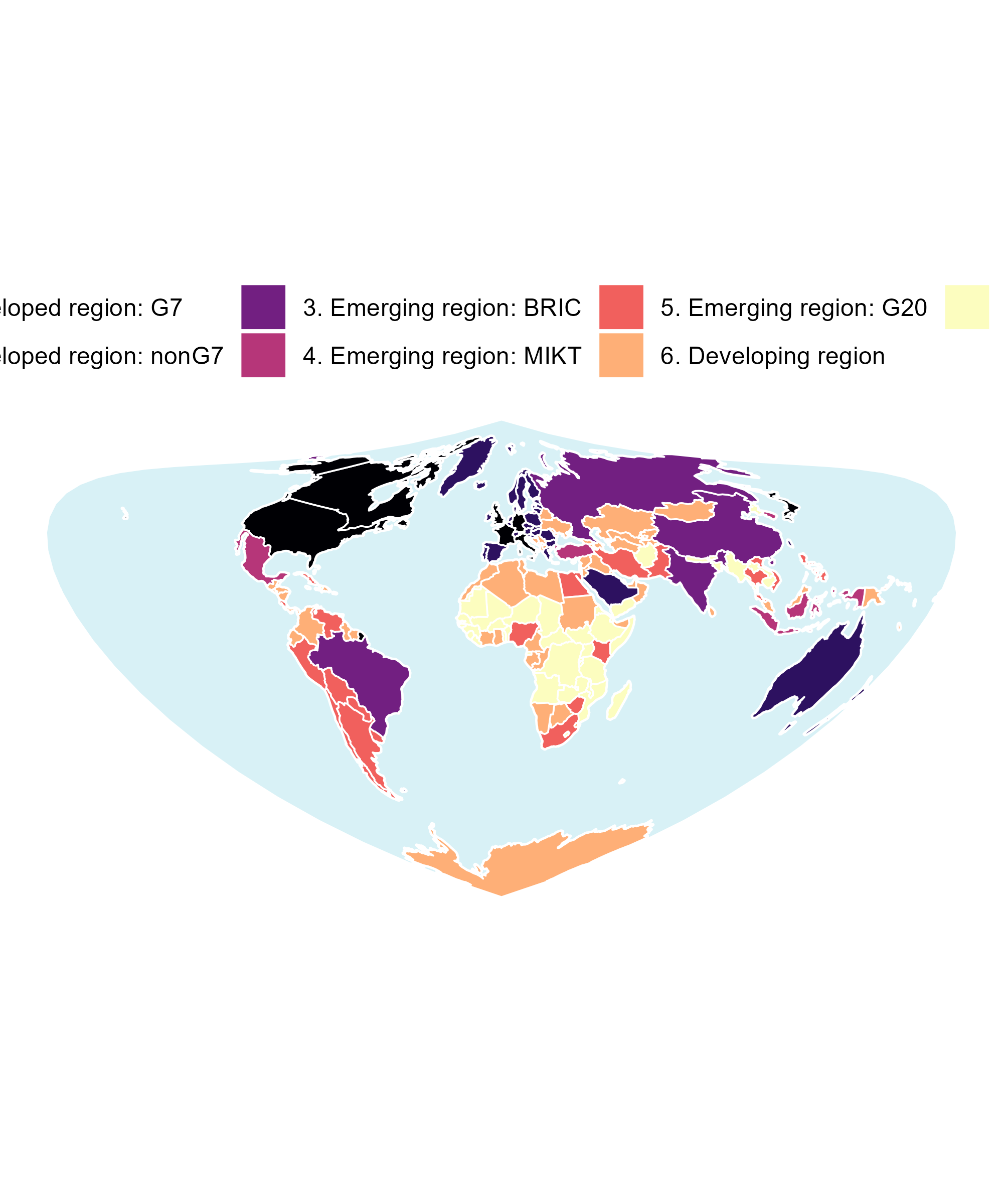
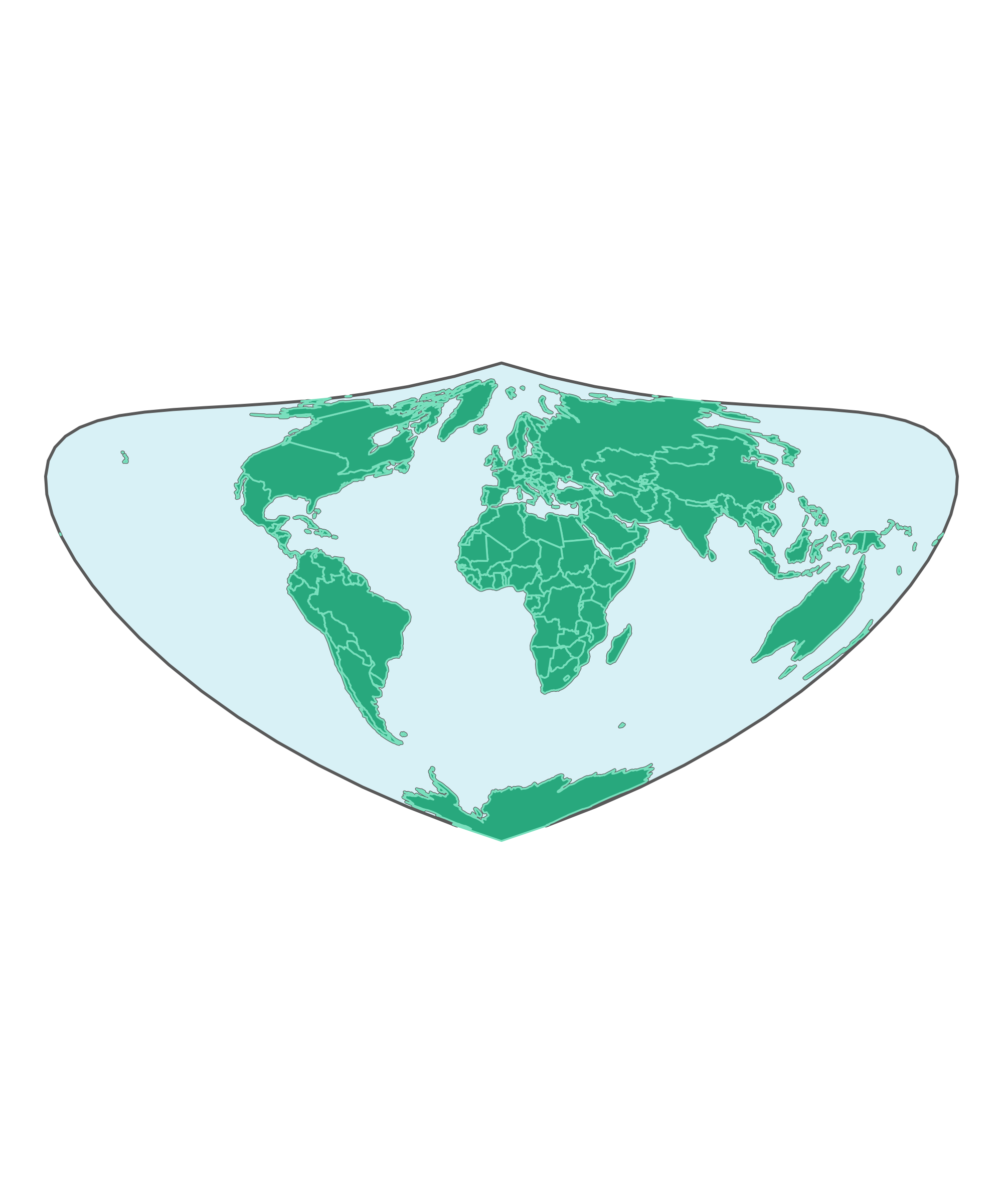
Better Borders
borders <- rmapshaper::ms_innerlines(countries)

ggplot() +
  geom_sf(
    data = oceans,
    fill = "#d8f1f6",
    color = "white"
  ) +
  geom_sf(
    data = countries,
    aes(fill = economy),
    color = "transparent"
  ) +
  geom_sf(
    data = borders,
    fill = "transparent",
    color = "white",
    size = .3
  ) +
  coord_sf(
    crs = "+proj=bonne +lat_1=10"
  ) +
  scale_fill_viridis_d(option = "magma") +
  theme_void() +
  theme(legend.position = "top")