library(tidyverse)

bikes <- readr::read_csv(
  here::here("data", "london-bikes-custom.csv"),
  col_types = "Dcfffilllddddc"
)

#bikes$season <- factor(bikes$season, levels = c("spring", "summer", "autumn", "winter"))
bikes$season <- forcats::fct_inorder(bikes$season)

theme_set(theme_light(base_size = 14, base_family = "Roboto Condensed"))

theme_update(
  panel.grid.minor = element_blank(),
  legend.position = "top"
)Graphic Design with ggplot2
Working with Labels and Annotations
Working with Labels
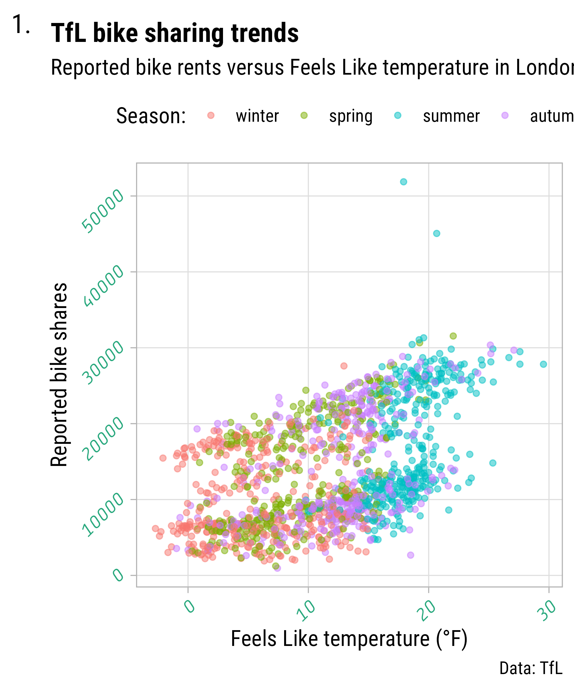
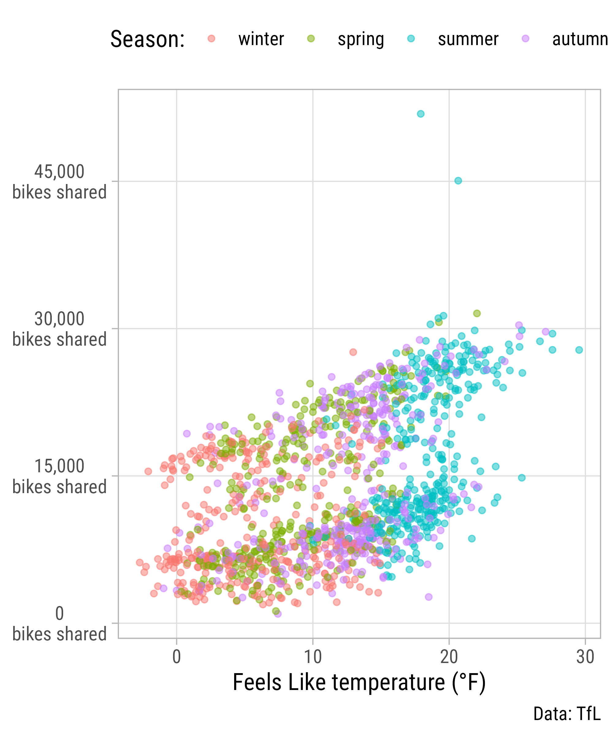
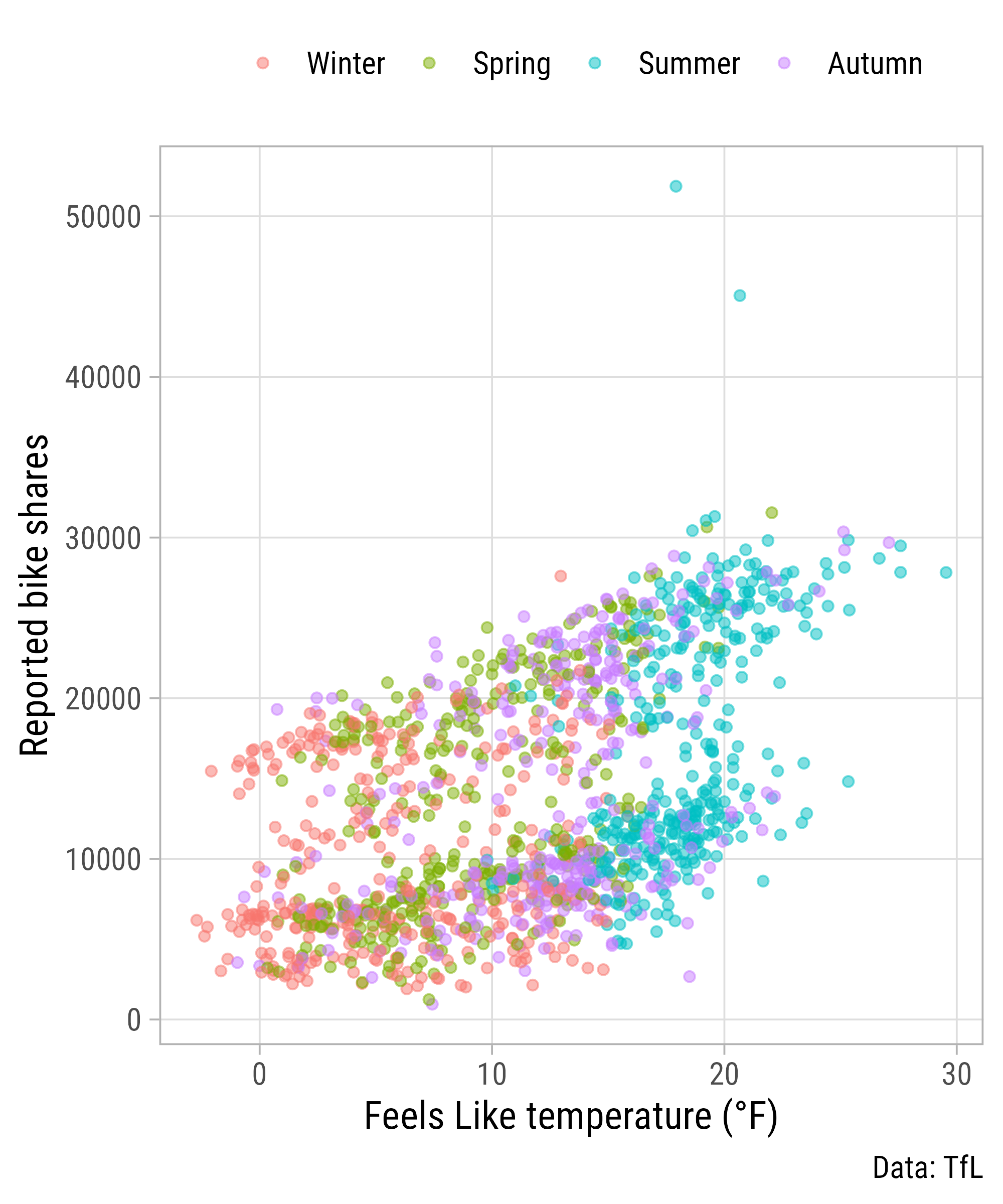
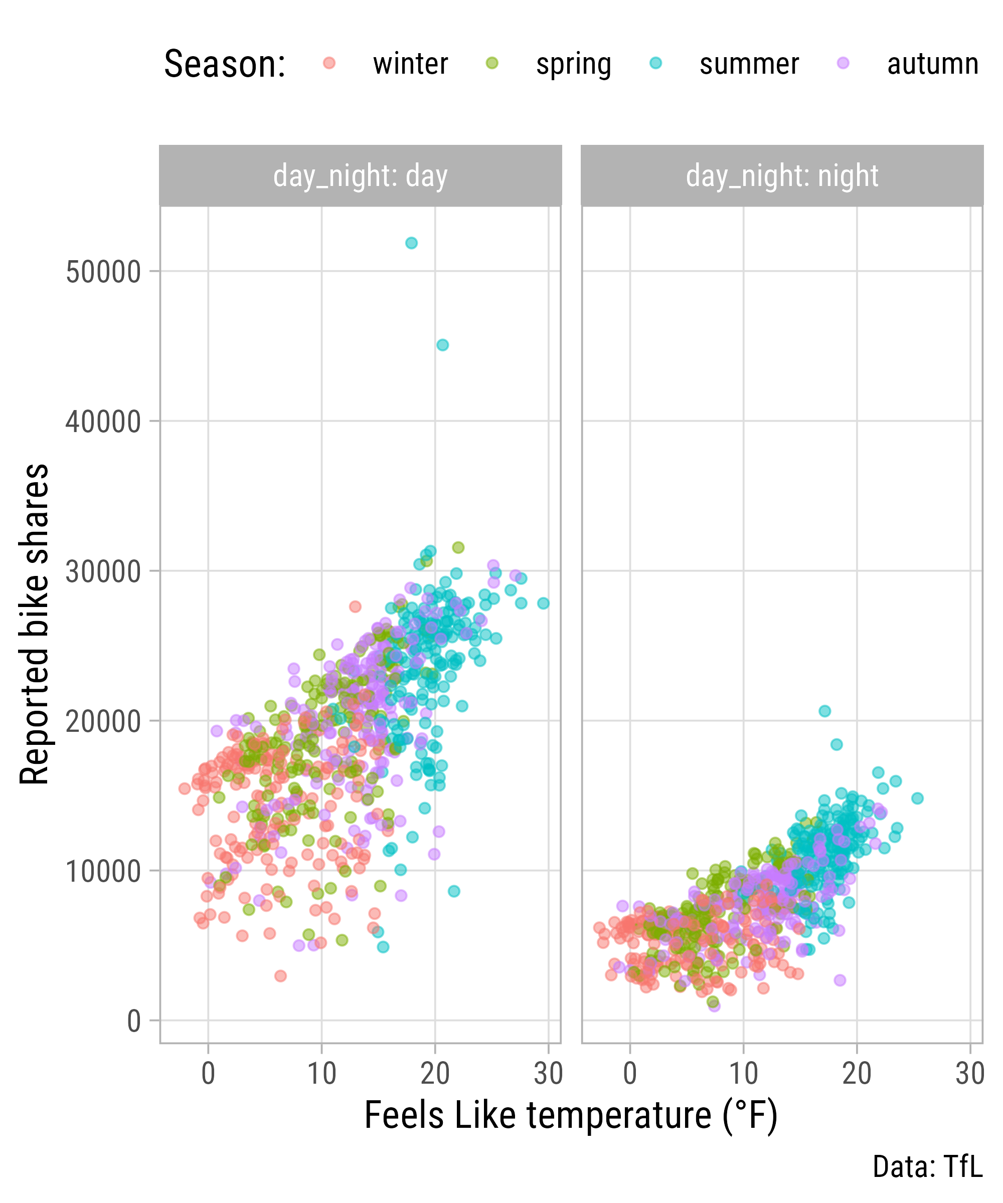
g <- ggplot(
    bikes,
    aes(x = temp_feel, y = count,
        color = season)
  ) +
  geom_point(
    alpha = .5
  ) +
  labs(
    x = "Feels Like temperature (°F)",
    y = "Reported bike shares",
    title = "TfL bike sharing trends",
    subtitle = "Reported bike rents versus Feels Like temperature in London",
    caption = "Data: TfL",
    color = "Season:",
    tag = "1."
  )

g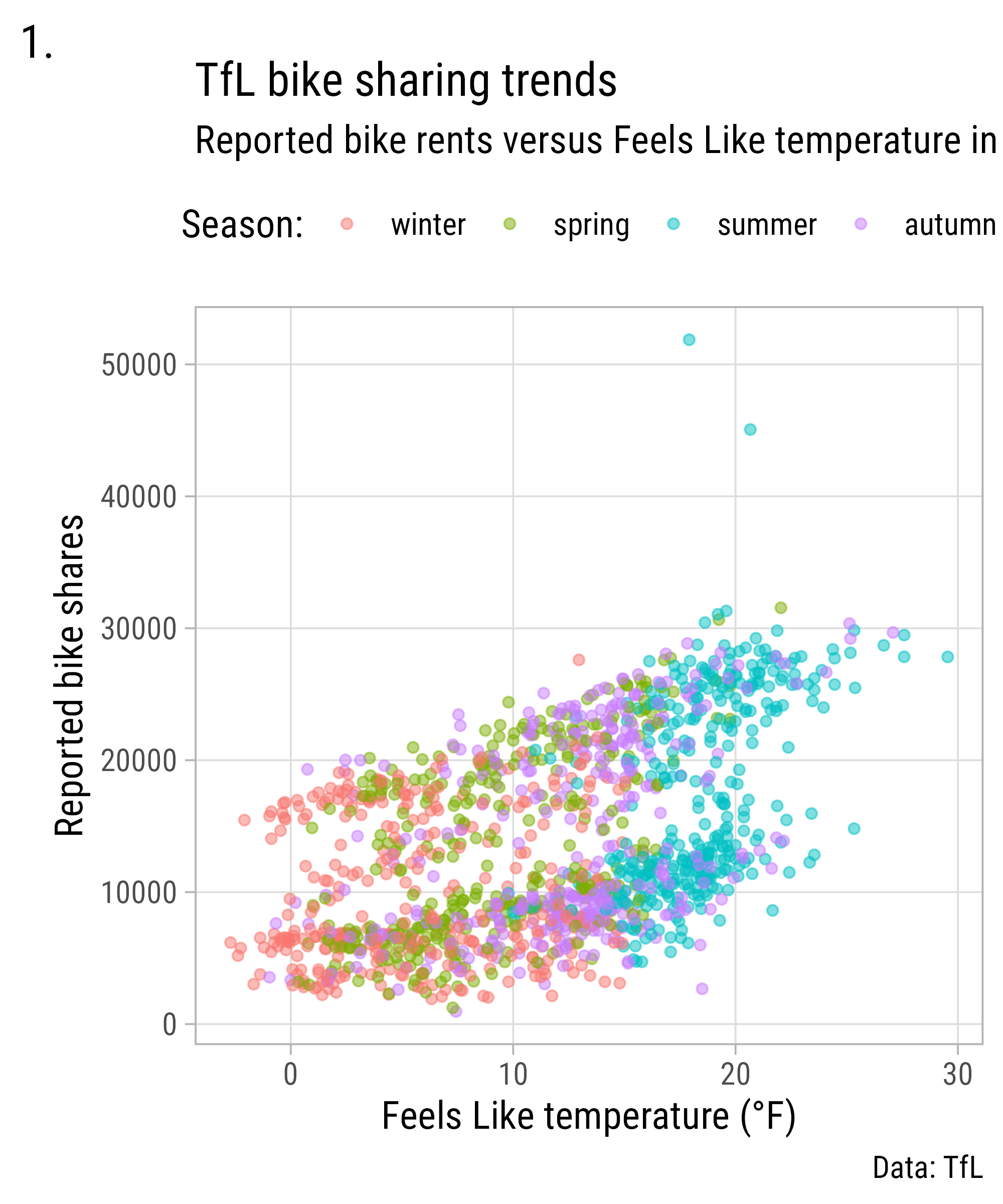
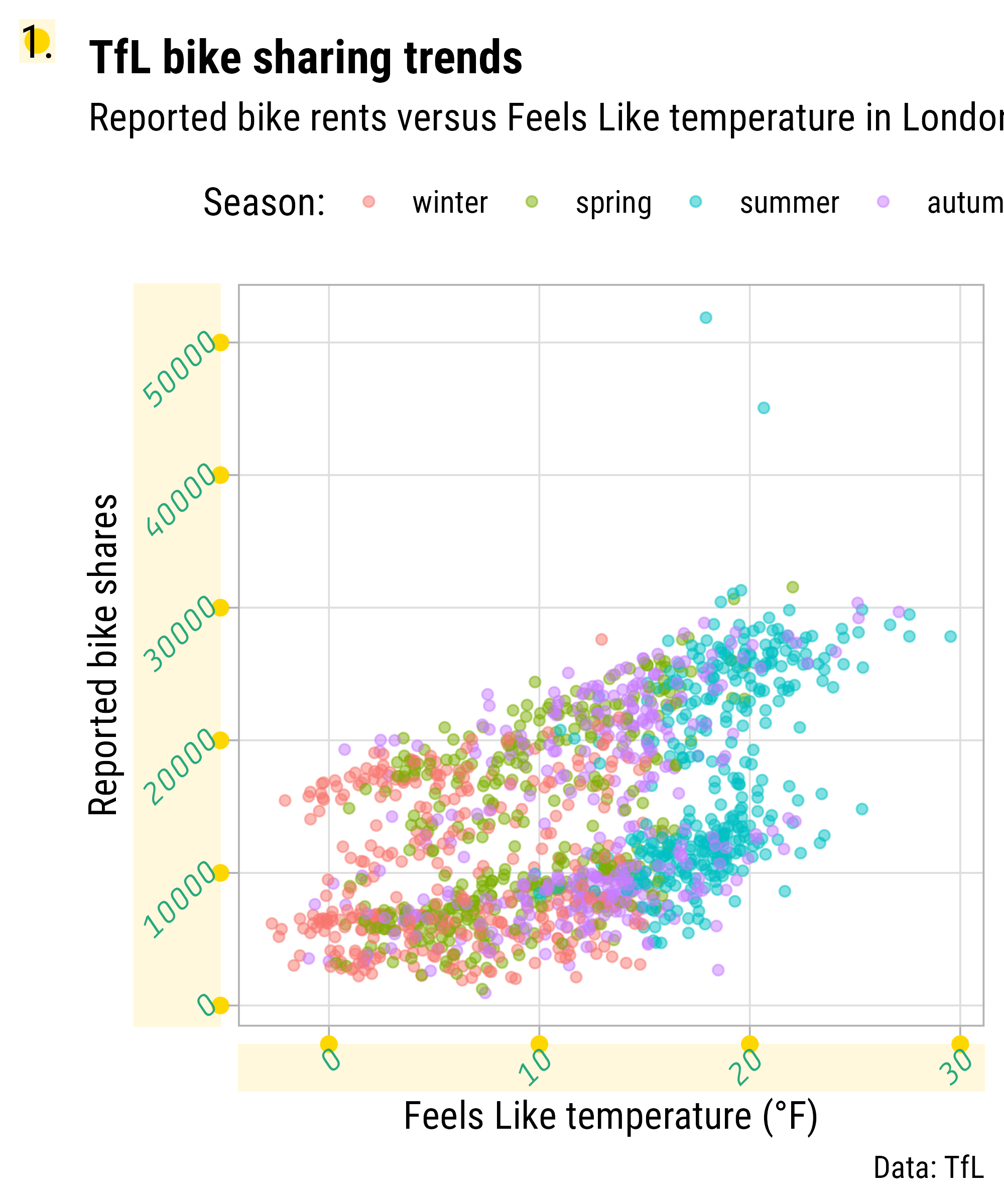
Customize Labels via `theme()`

Customize Labels via `theme()`
Customize Labels via `theme()`
Customize Labels via `theme()`
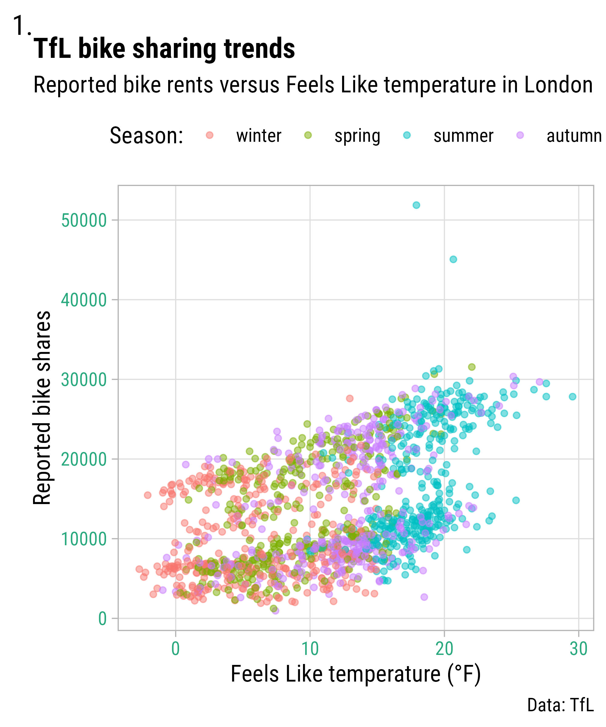
g + theme(
  plot.title = element_text(face = "bold"),
  plot.title.position = "plot",
  axis.text = element_text(
    color = "#28a87d",
    family = "Tabular",
    face = "italic",
    colour = NULL,
    size = NULL,
    hjust = 1,
    vjust = 0,
    angle = 45,
    lineheight = 1.3, ## no effect here
    margin = margin(10, 0, 20, 0) ## no effect here
  ),
  axis.text.x = element_text(
    margin = margin(10, 0, 20, 0) ## trbl
  )
)
Customize Labels via `theme()`
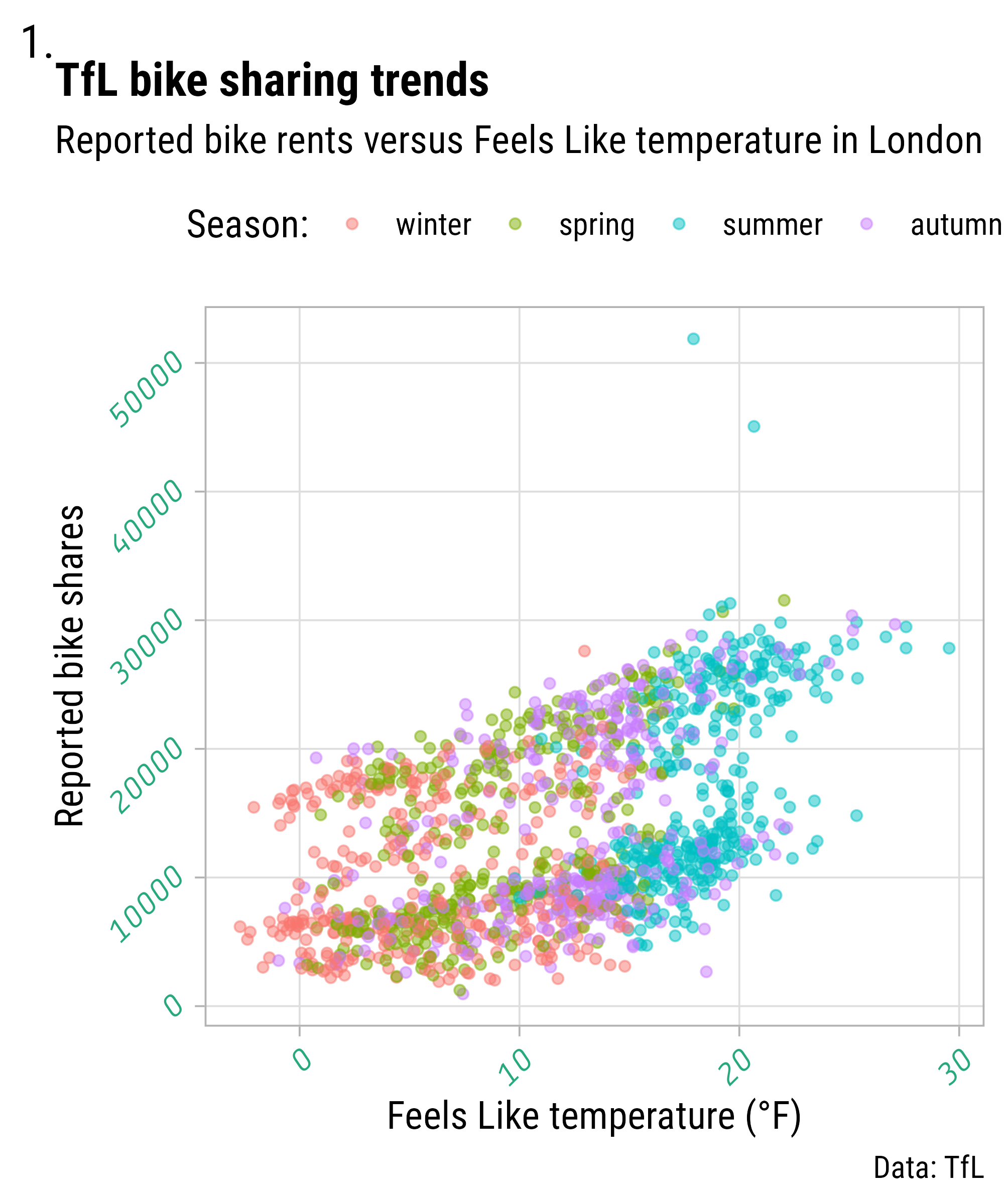
g + theme(
  plot.title = element_text(face = "bold"),
  plot.title.position = "plot",
  axis.text = element_text(
    color = "#28a87d",
    family = "Tabular",
    face = "italic",
    colour = NULL,
    size = NULL,
    hjust = 1,
    vjust = 0,
    angle = 45,
    lineheight = 1.3, ## no effect here
    margin = margin(10, 0, 20, 0) ## no effect here
  ),
  plot.tag = element_text(
    margin = margin(0, 12, -8, 0) ## trbl
  )
)
Customize Labels via `theme()`
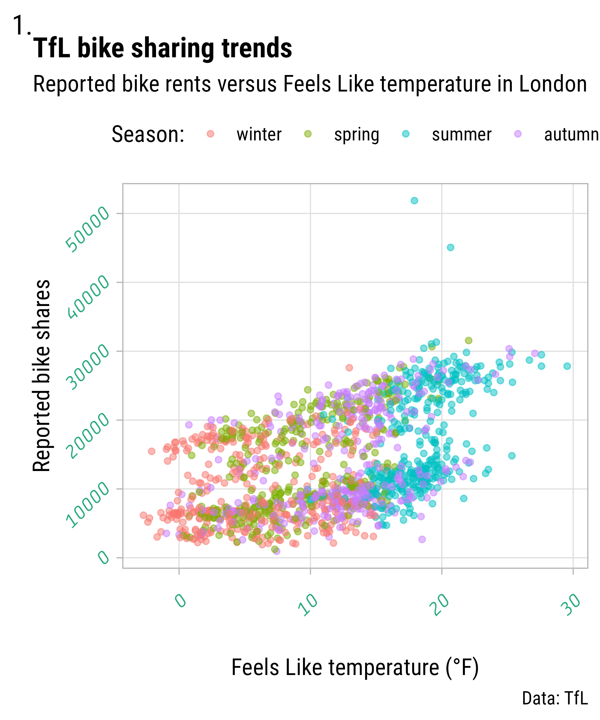
g + theme(
  plot.title = element_text(face = "bold"),
  plot.title.position = "plot",
  axis.text = element_text(
    color = "#28a87d",
    family = "Tabular",
    face = "italic",
    colour = NULL,
    size = NULL,
    hjust = 1,
    vjust = 0,
    angle = 45,
    lineheight = 1.3, ## no effect here
    margin = margin(10, 0, 20, 0), ## no effect here
    debug = TRUE
  ),
  plot.tag = element_text(
    margin = margin(0, 12, -8, 0), ## trbl
    debug = TRUE
  )
)
Format Labels via `scale_*`
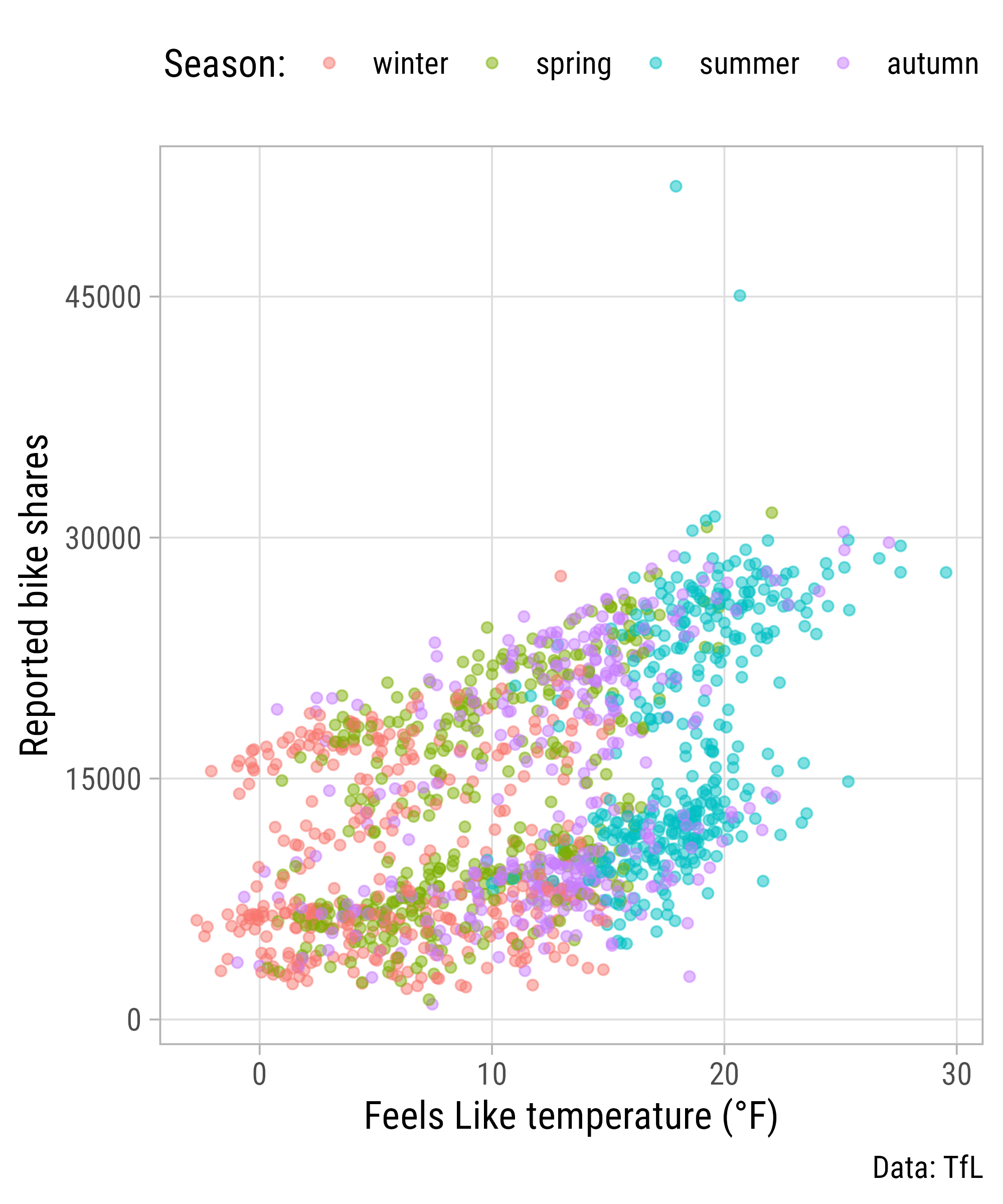
Format Labels via `scale_*`

Format Labels via `scale_*`
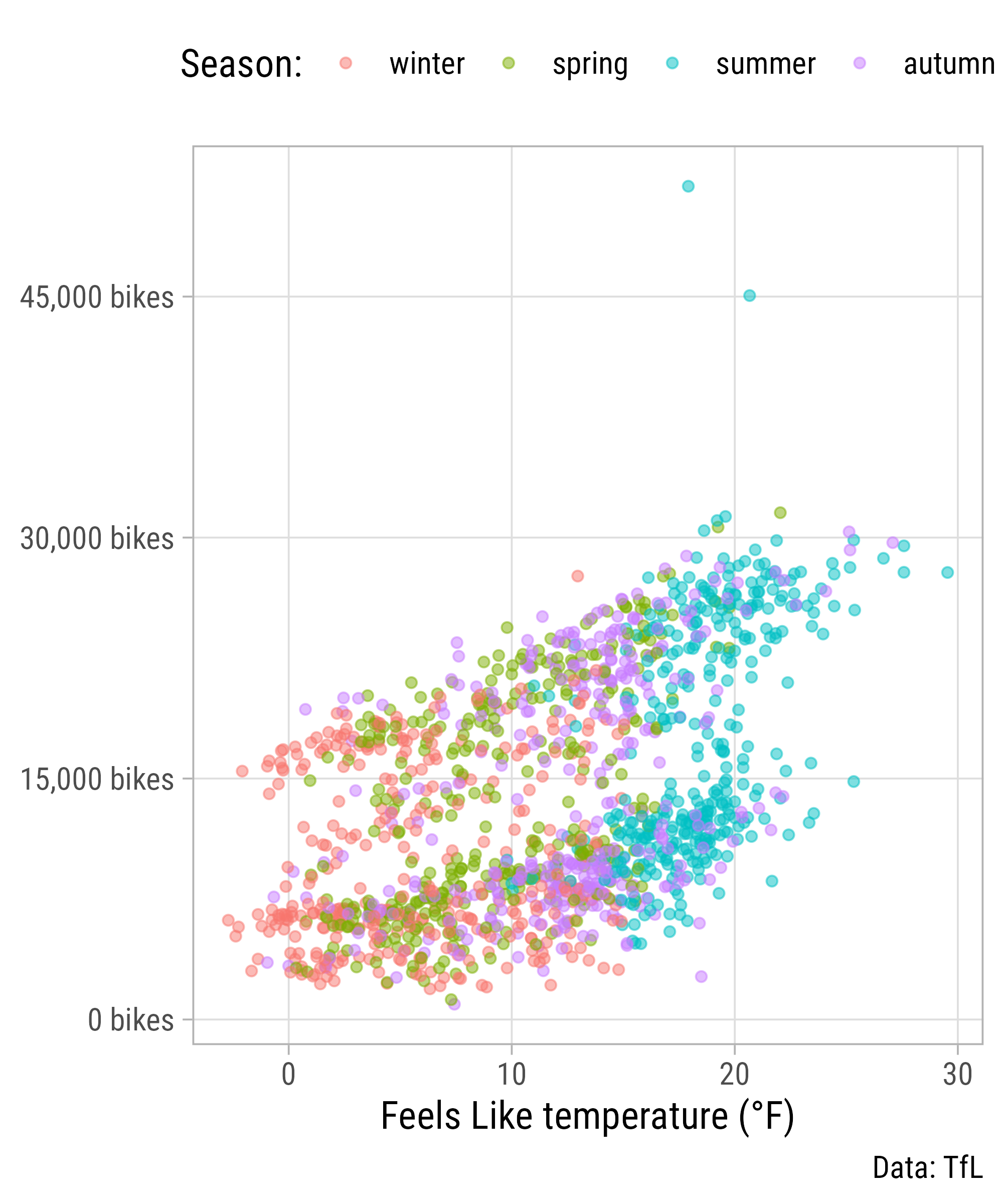
Format Labels via `scale_*`
Format Labels via `scale_*`
Format Labels via `scale_*`

Format Labels via `scale_*`

Format Labels via `scale_*`
Format Labels via `scale_*`
Format Labels via `scale_*`
Styling Labels with {ggtext}
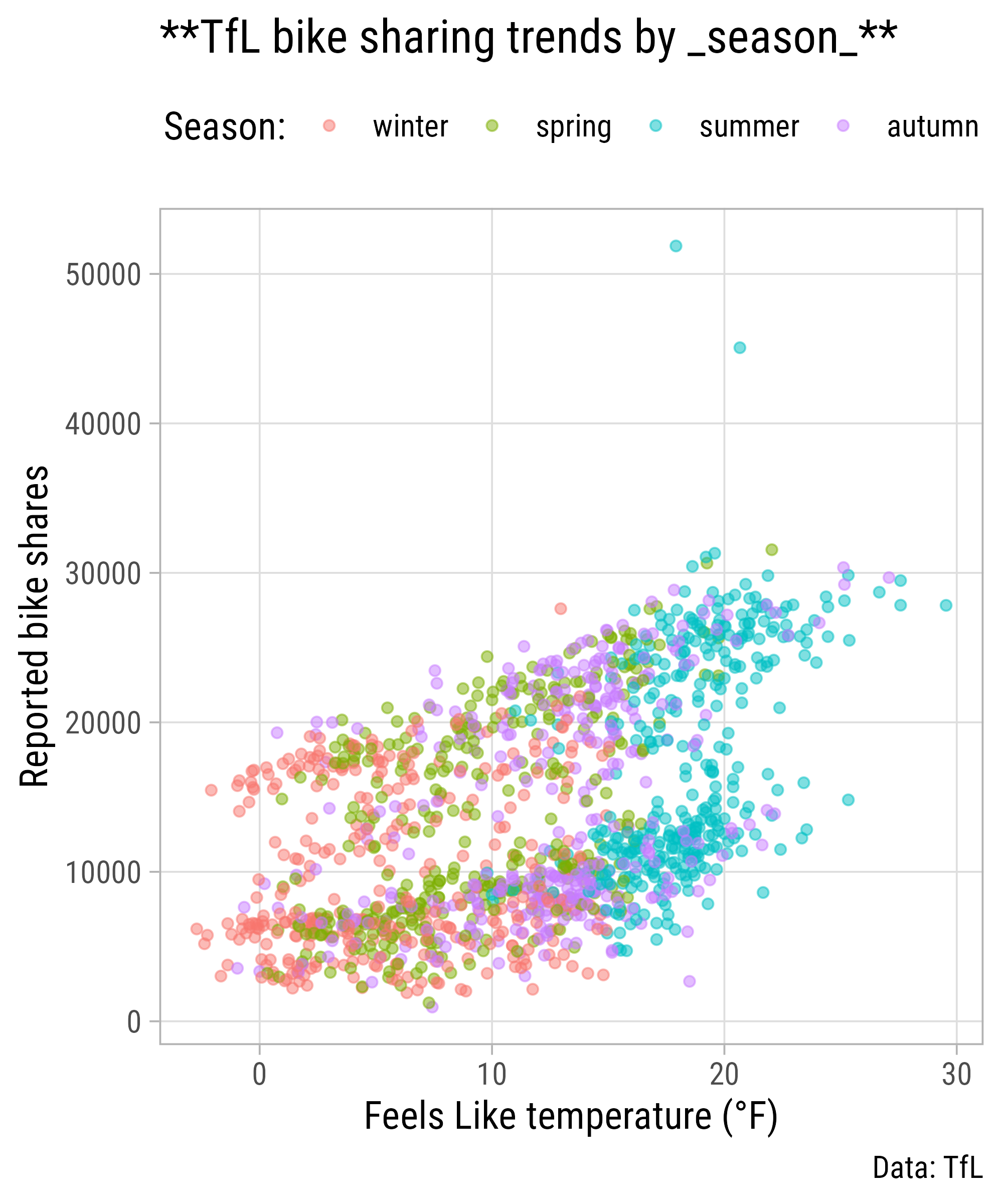
Styling Labels with {ggtext}
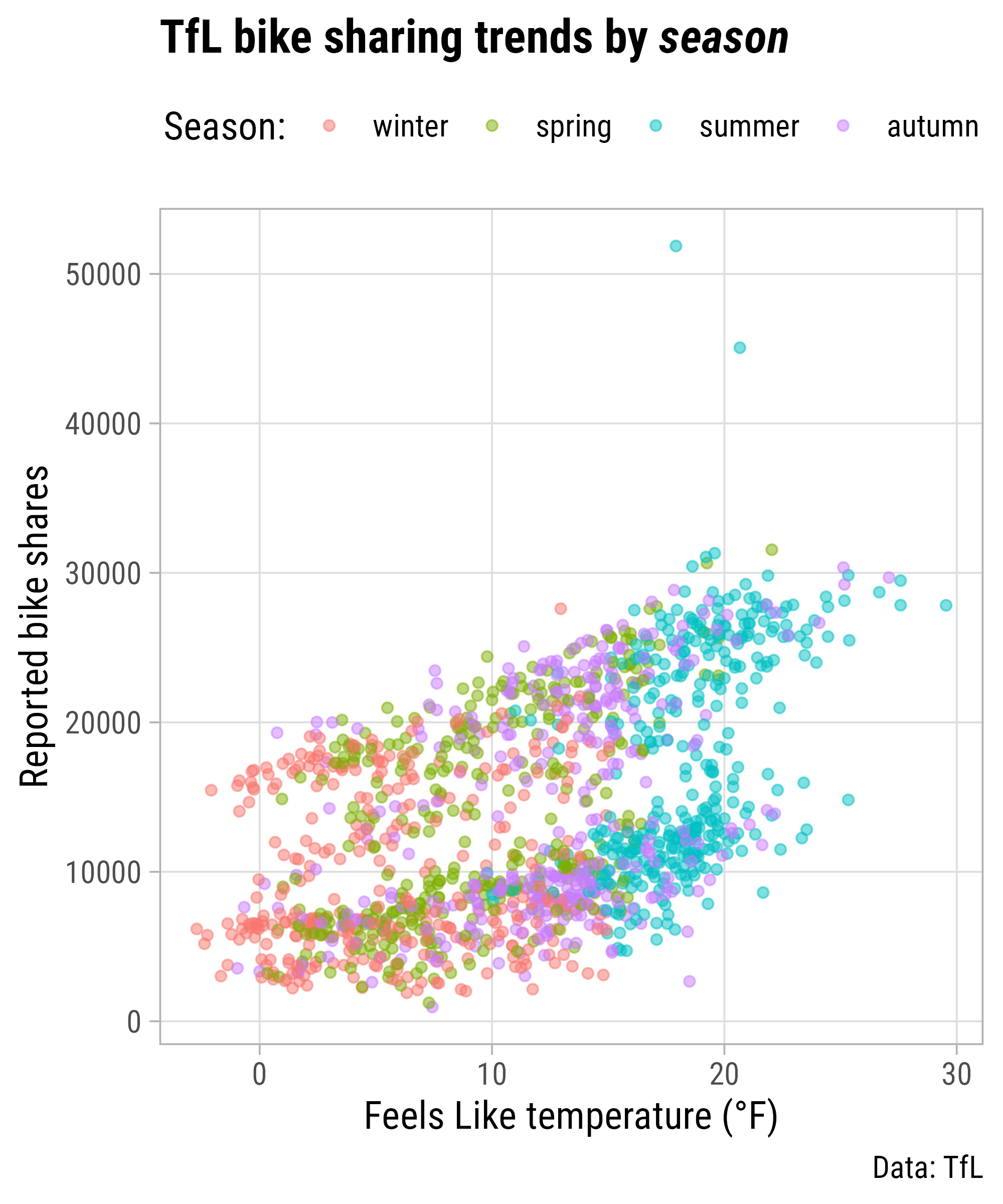
Styling Labels with {ggtext}
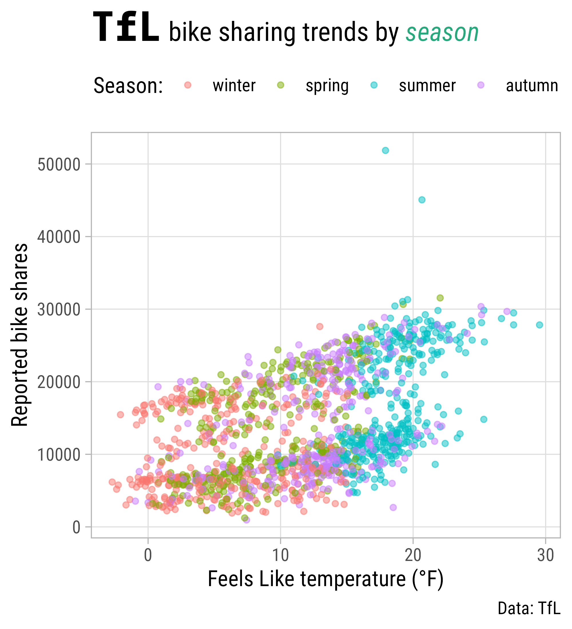
<b style='font-family:tabular;font-size:15pt;'>TfL</b> bike sharing trends by <i style='color:#28a87d;'>season</i>
Facet Labellers
Facet Labellers

Facet Labellers
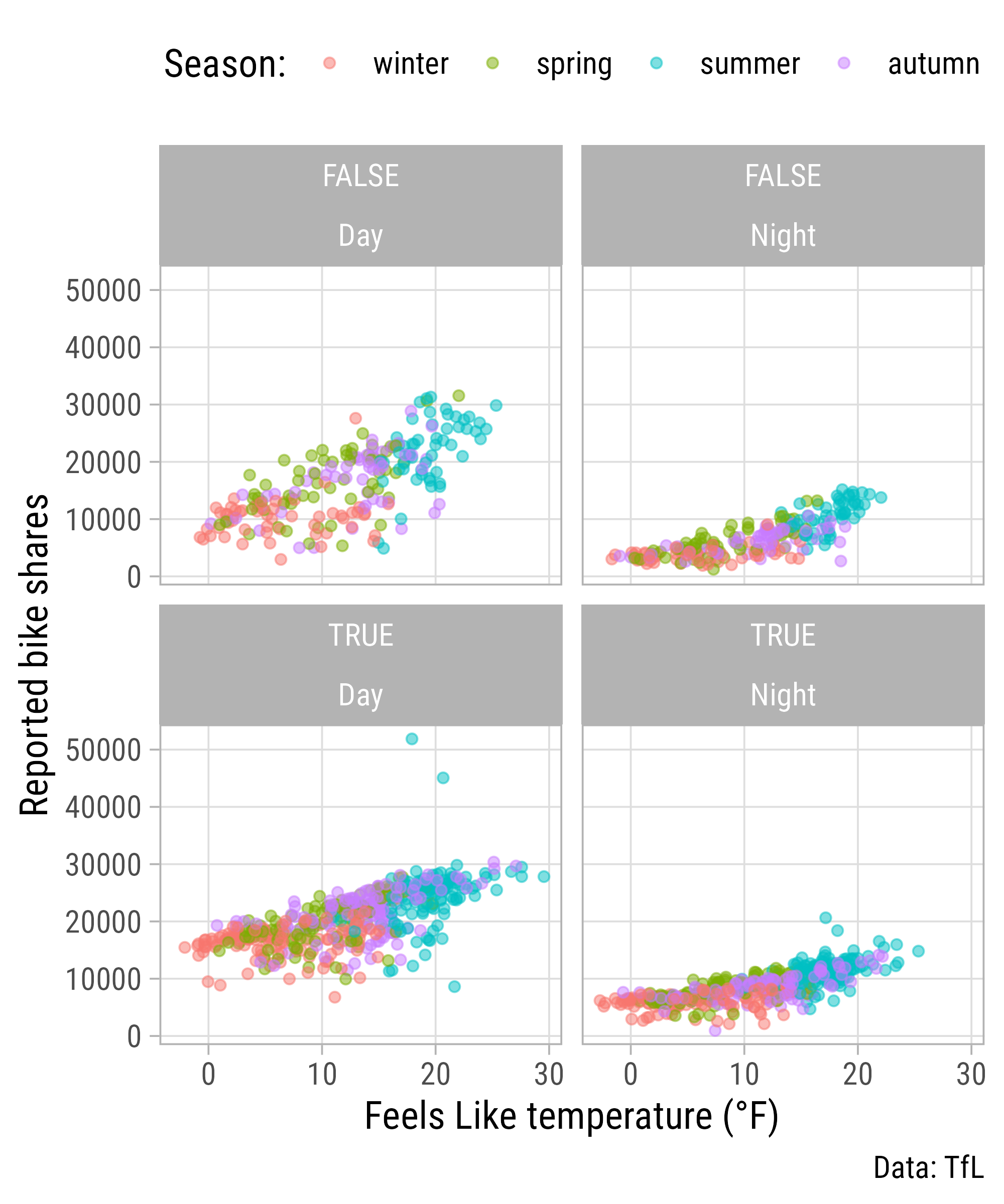
Facet Labellers

Facet Labellers
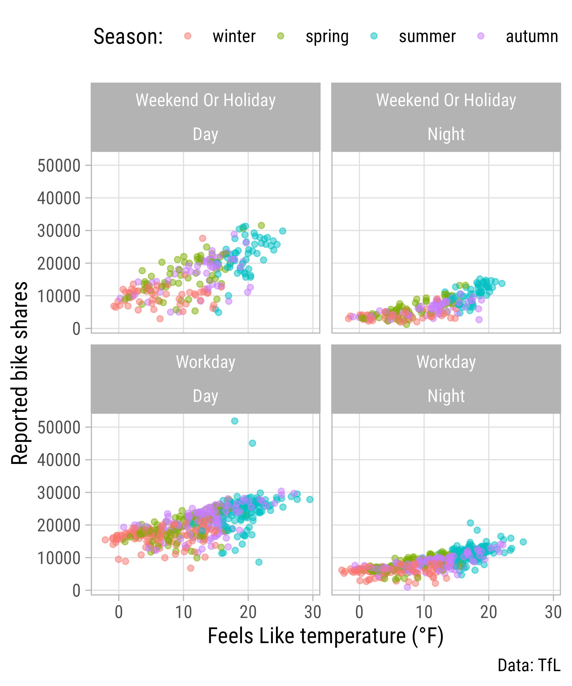
Facet Labeller

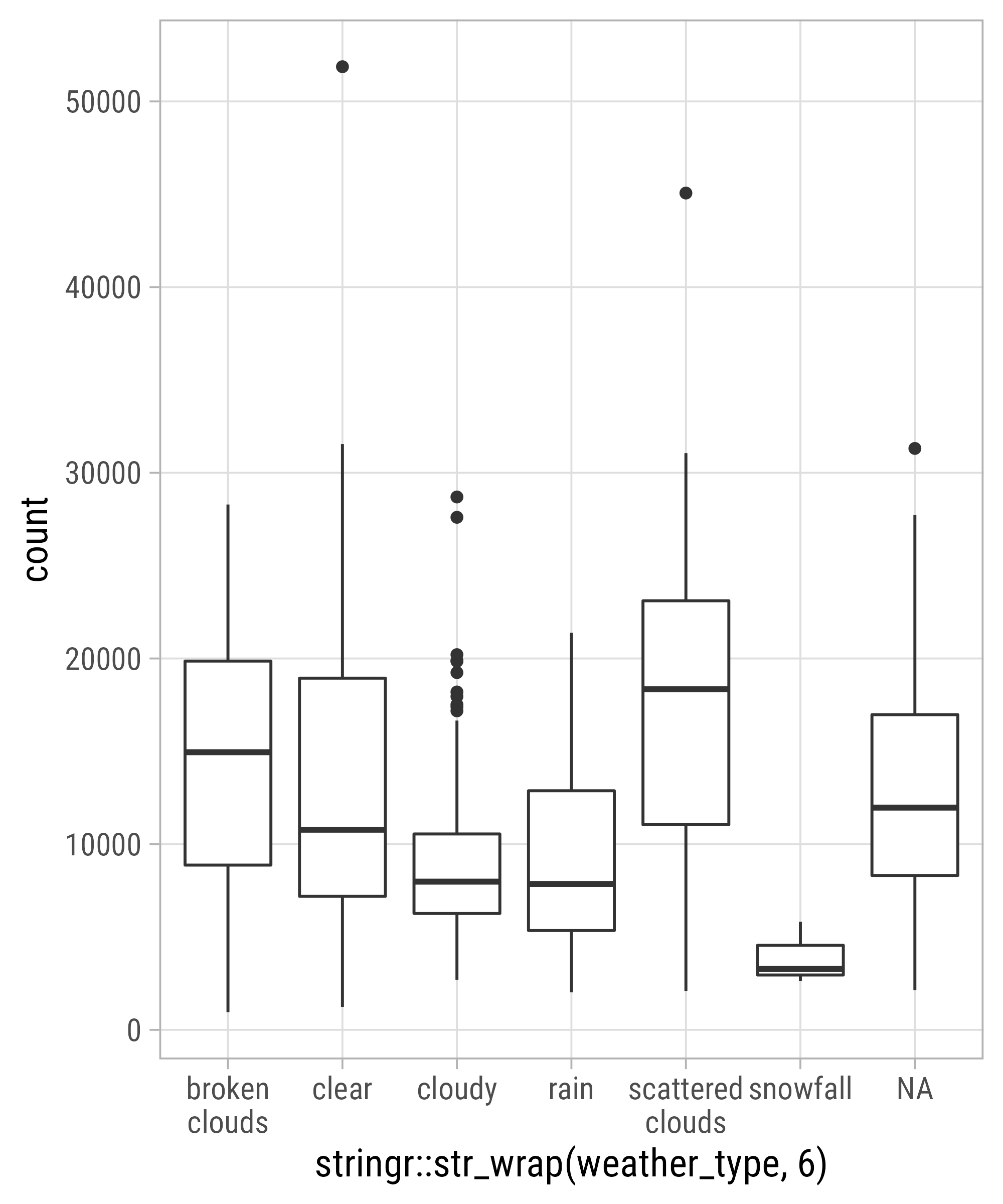
Handling Long Labels with {stringr}
Handling Long Labels with {stringr}
Handling Long Labels with {ggtext}
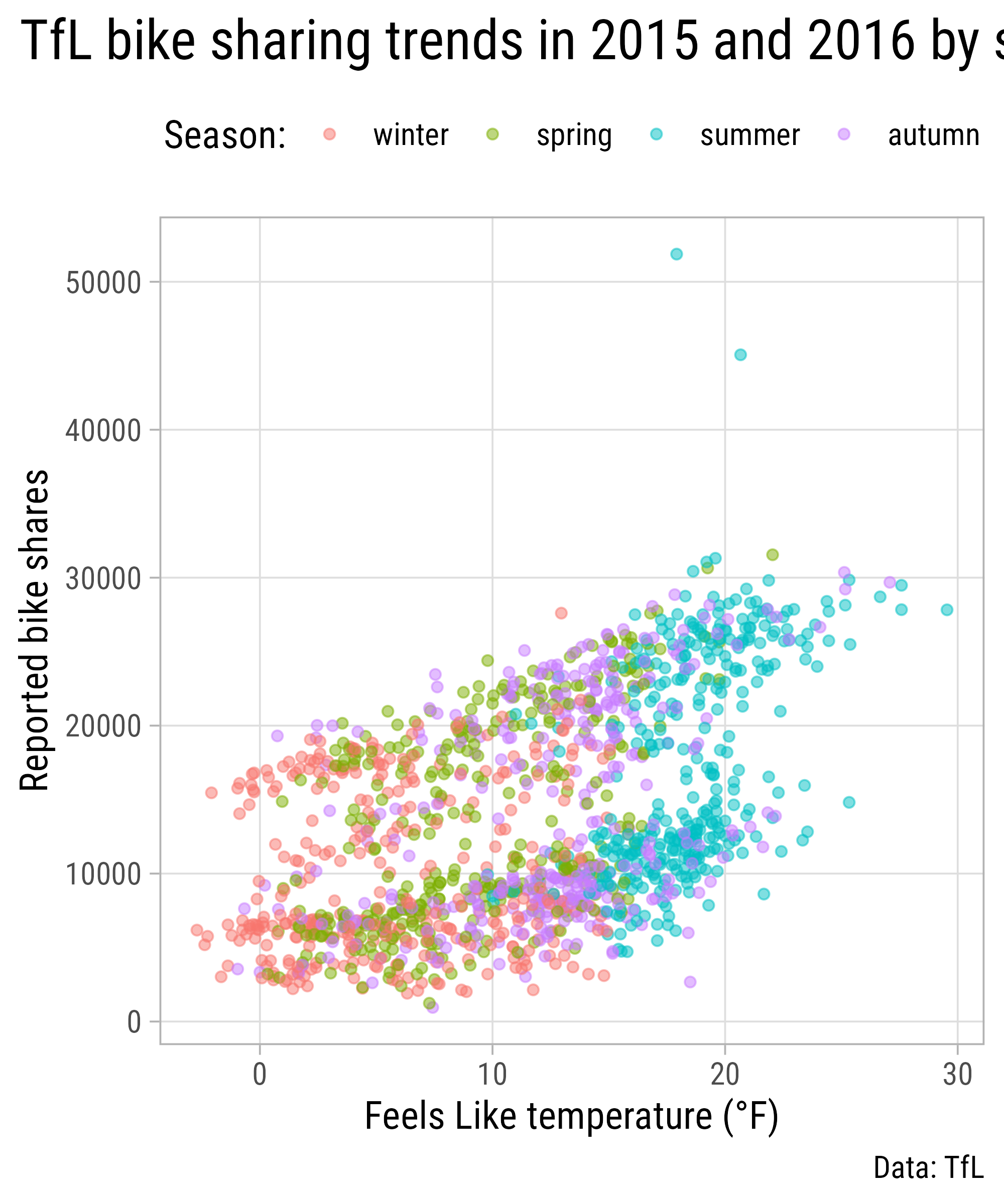
Handling Long Titles
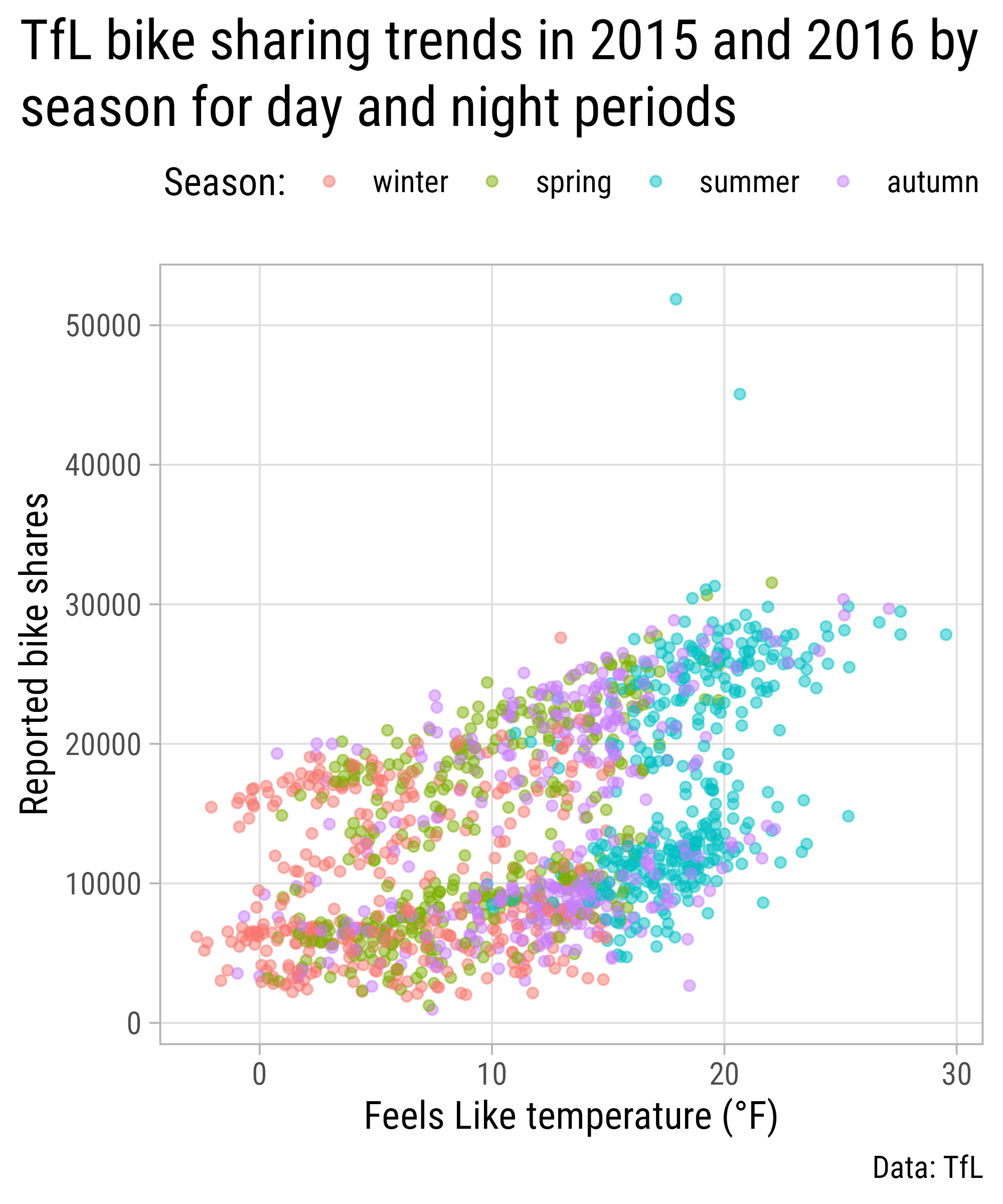
Handling Long Titles
Handling Long Titles
Handling Long Titles
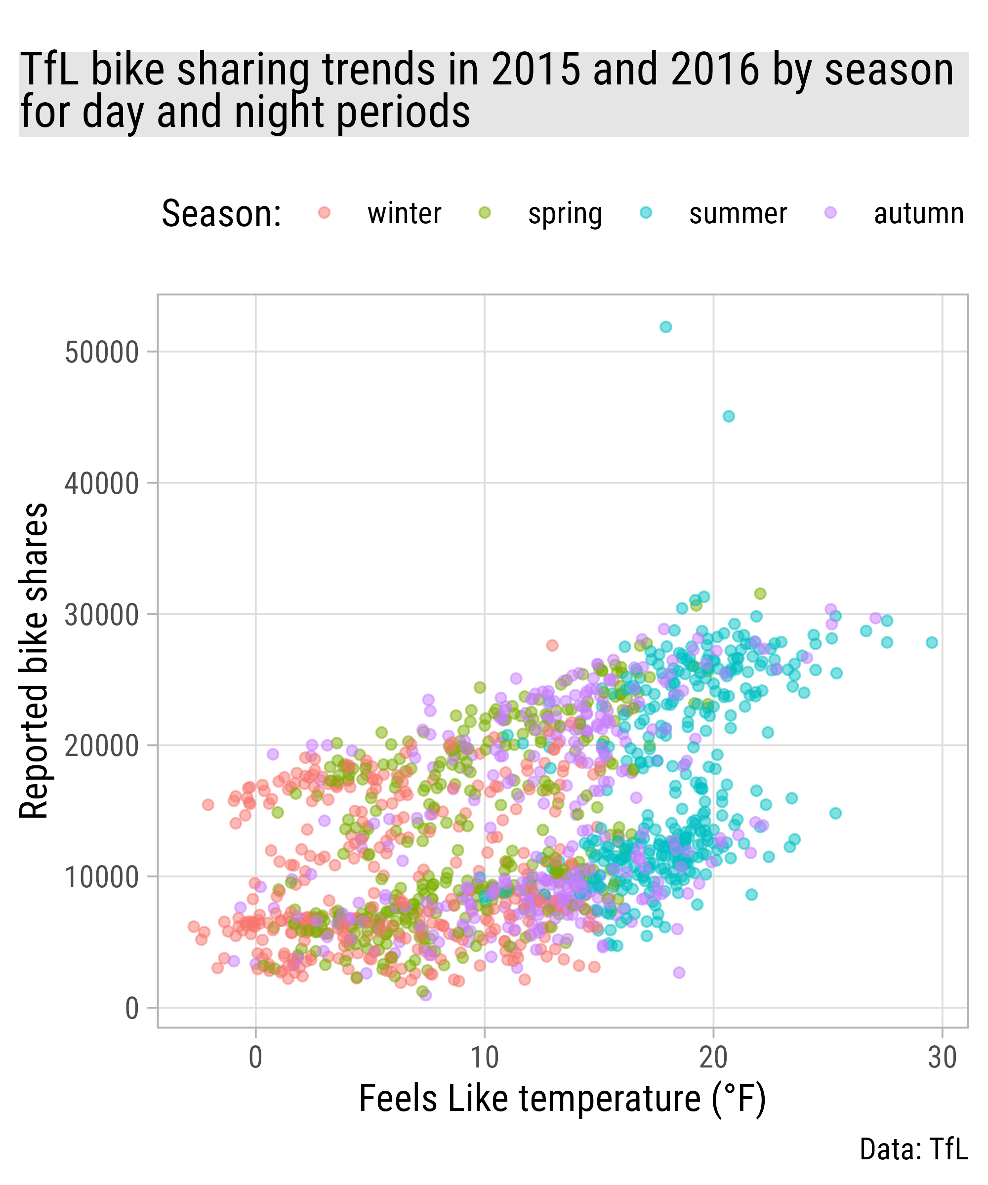
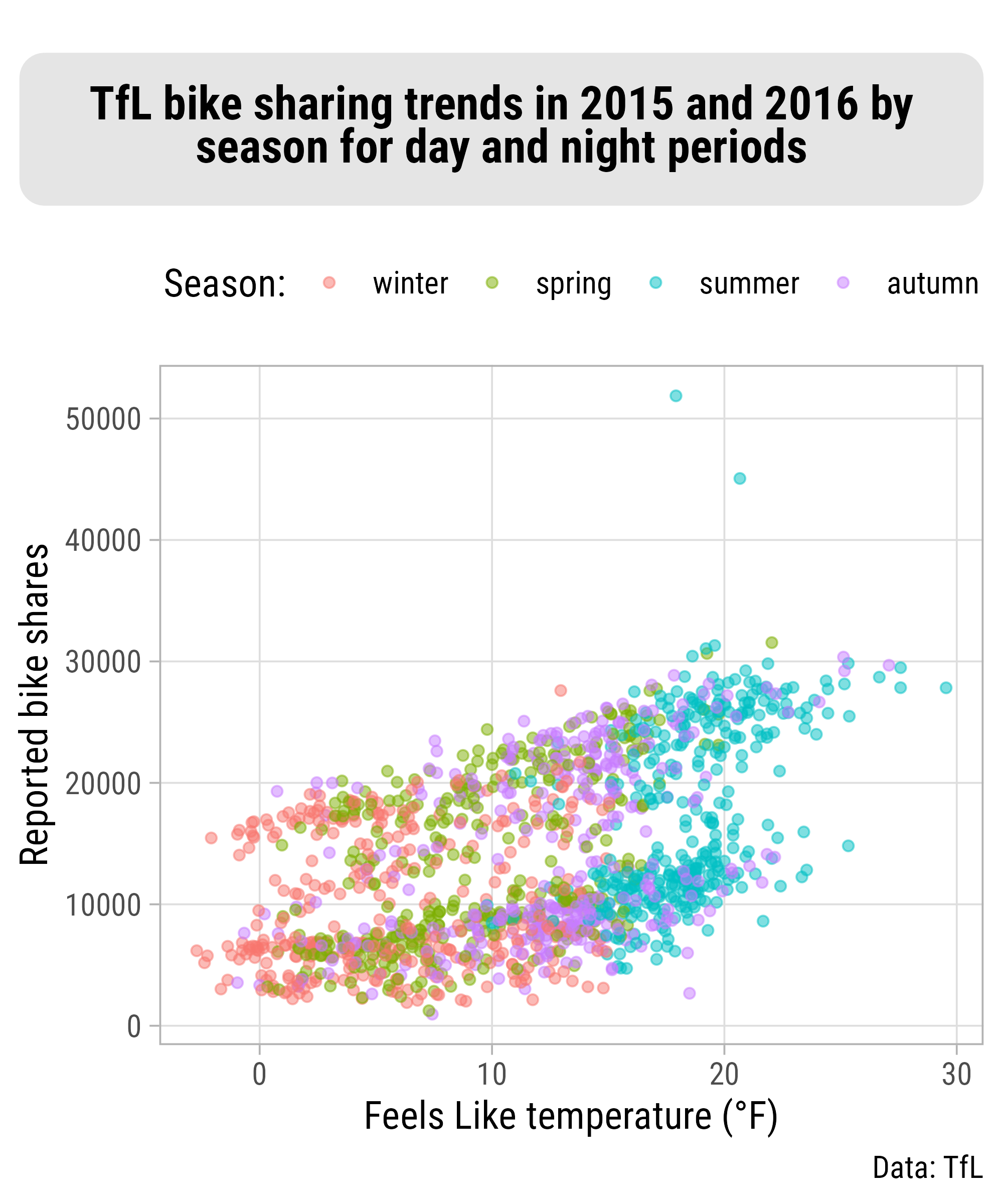
g +
  ggtitle("TfL bike sharing trends in 2015 and 2016 by season for day and night periods") +
  theme(
    plot.title = ggtext::element_textbox_simple(
      margin = margin(t = 12, b = 12),
      padding = margin(rep(12, 4)),
      fill = "grey90",
      box.color = "grey40",
      r = unit(9, "pt"),
      halign = .5,
      face = "bold",
      lineheight = .9
    ),
    plot.title.position = "plot"
  )
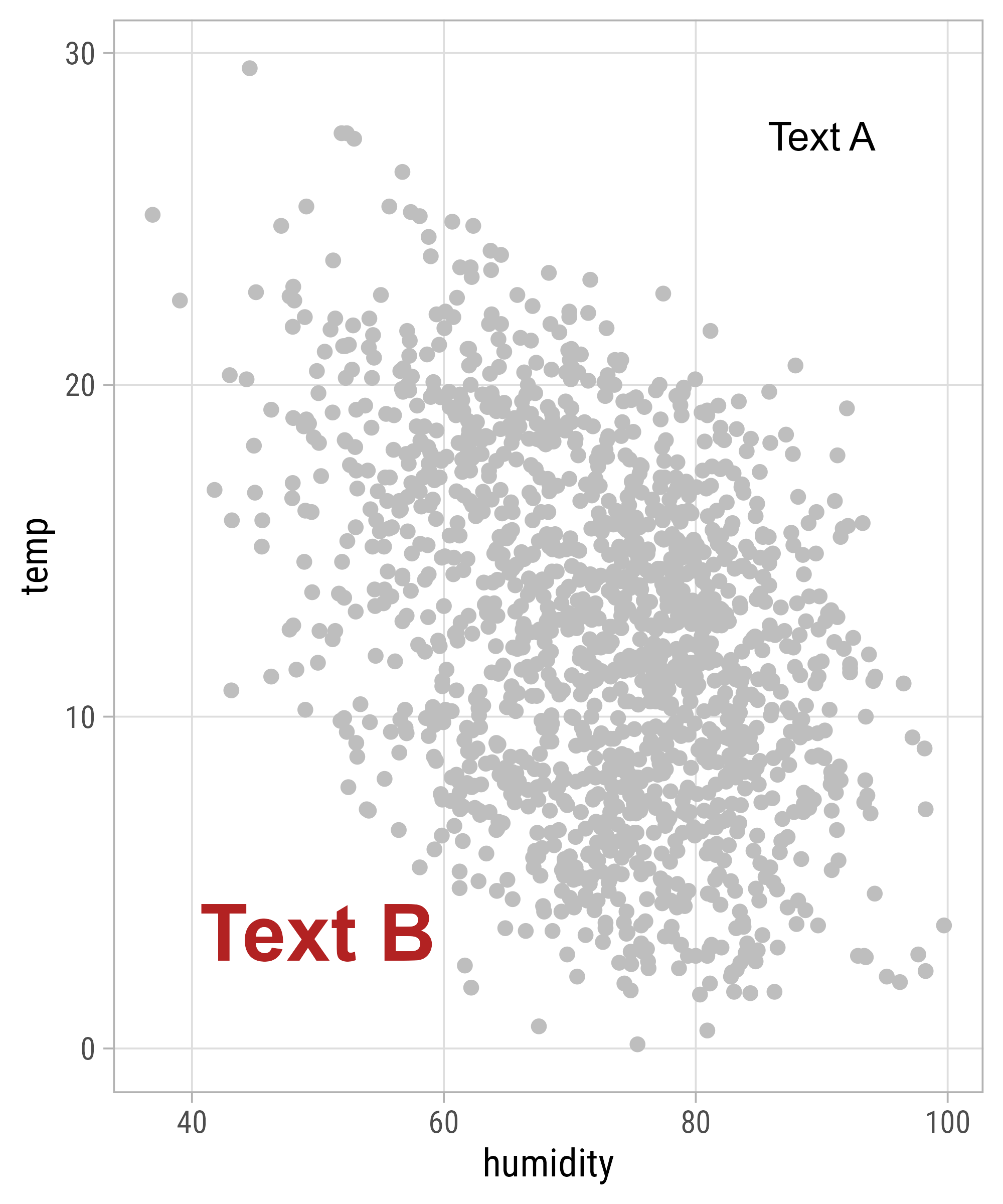
Add Single Text Annotations
Style Text Annotations
Add Multiple Text Annotations
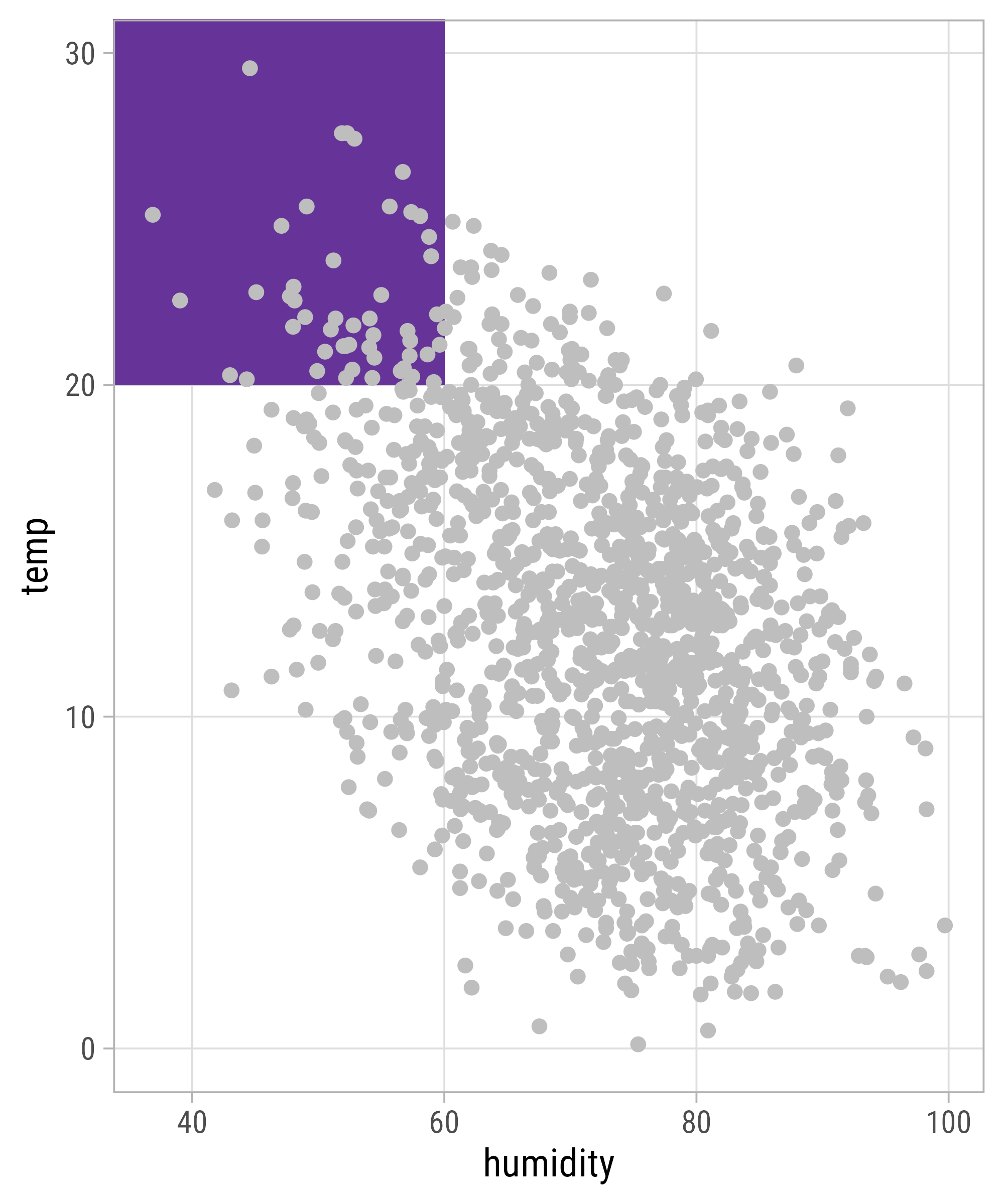
Add Boxes (Rectangles)
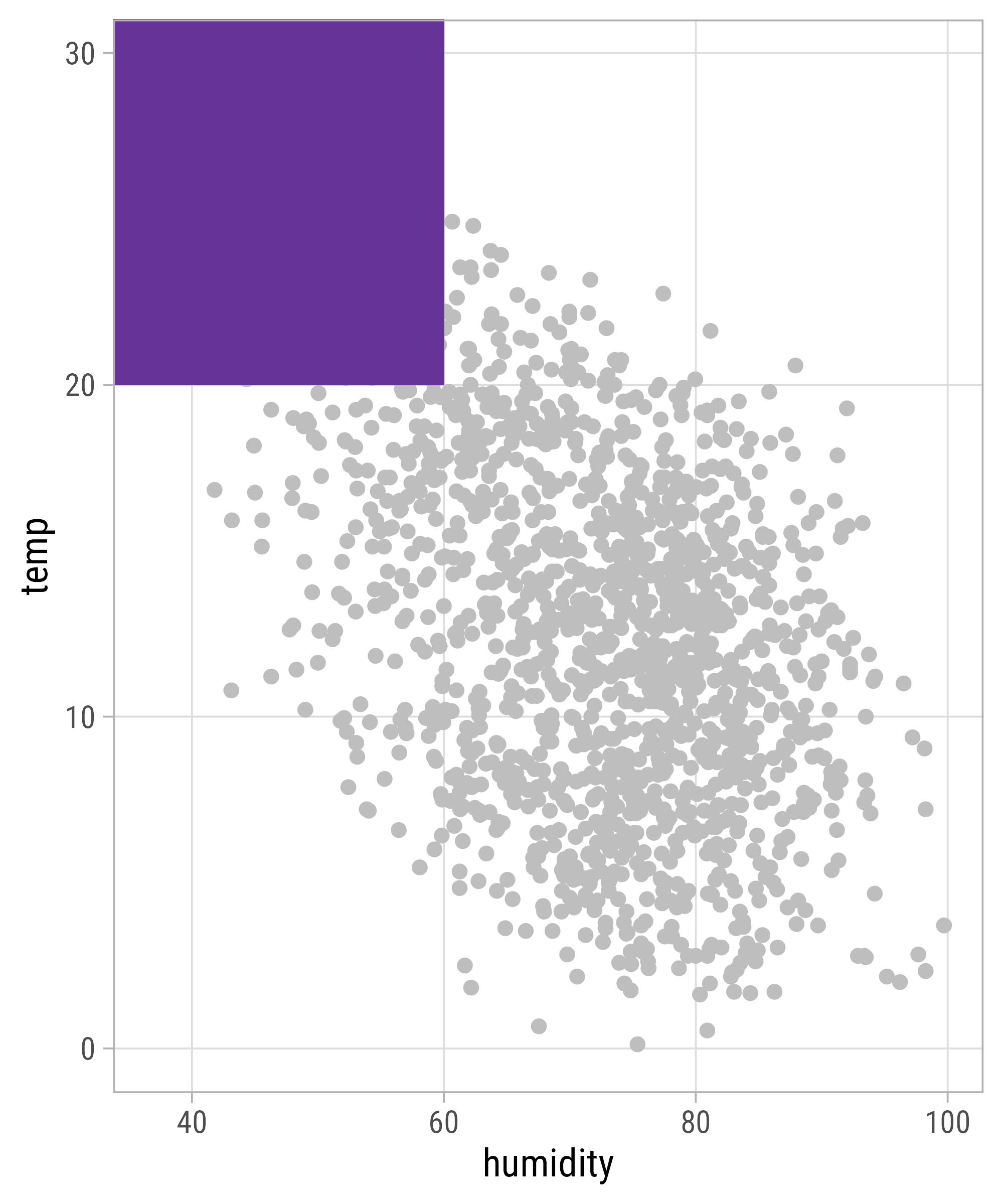
Add Boxes (Rectangles)
Add Lines (Segments)
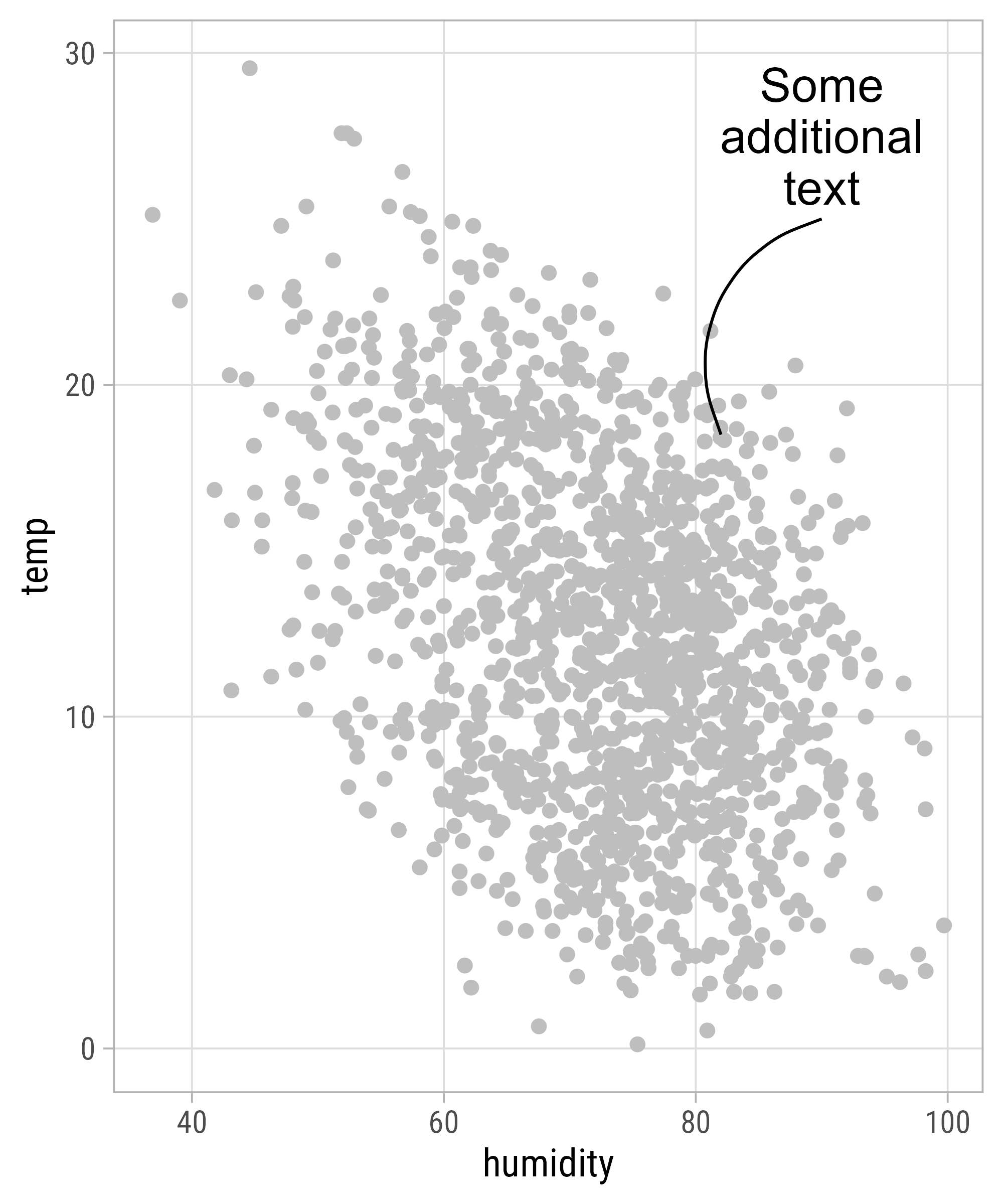
Add Curves
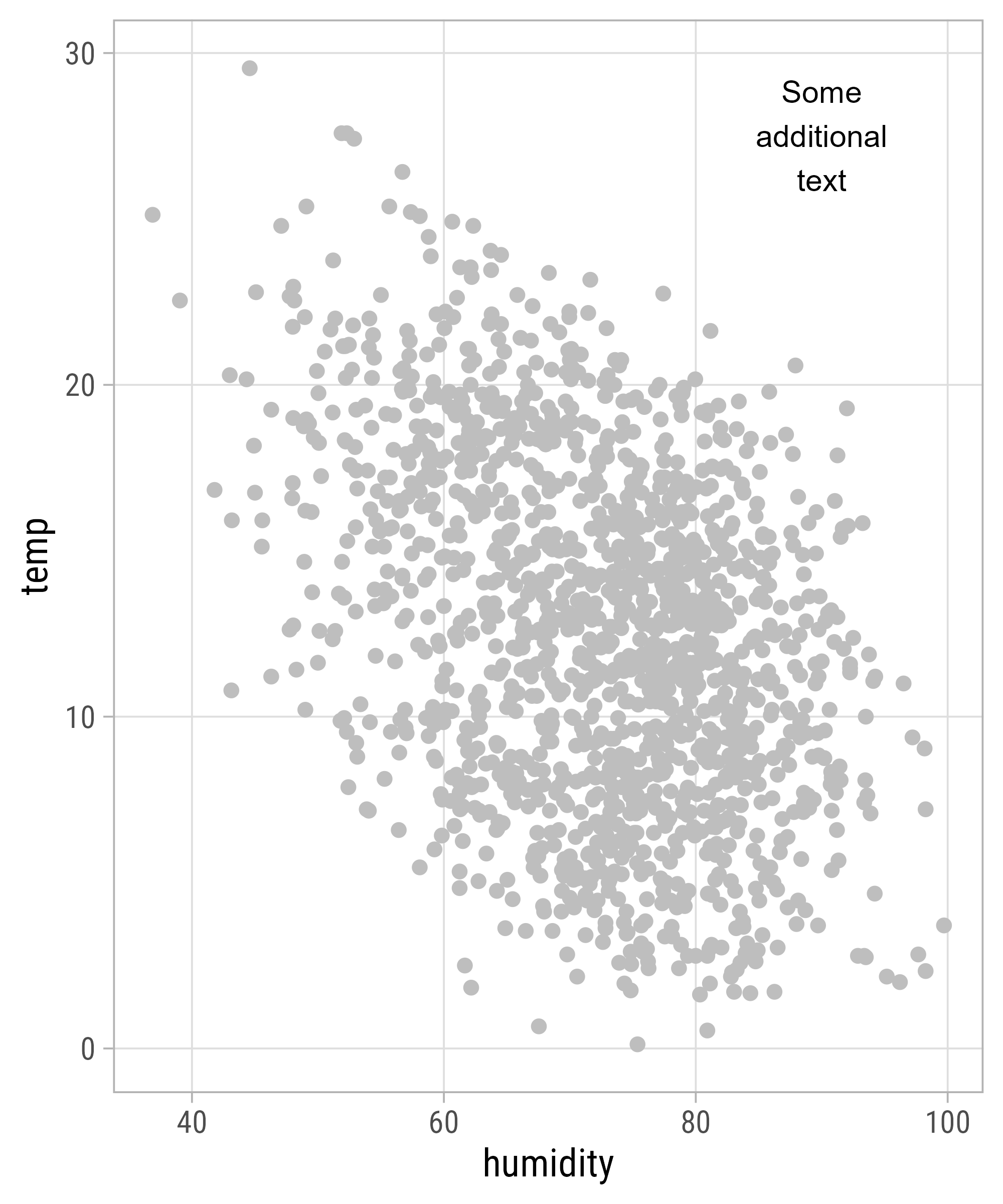
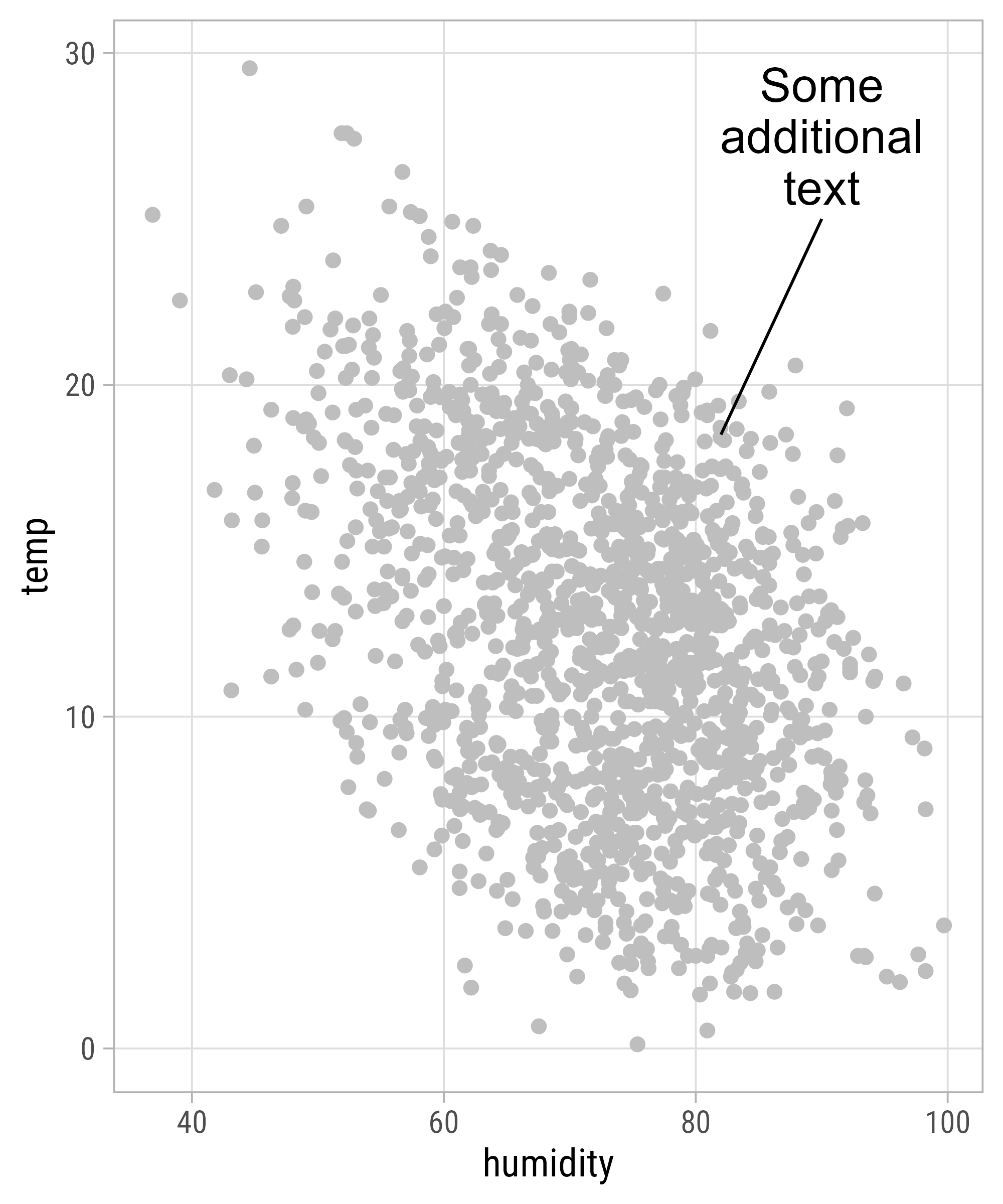
Add Arrows
Add Arrows
ggplot(bikes, aes(humidity, temp)) +
  geom_point(size = 2, color = "grey") +
  annotate(
    geom = "text",
    x = 90,
    y = 27.5,
    label = "Some\nadditional\ntext",
    size = 6,
    lineheight = .9
  ) +
  annotate(
    geom = "curve",
    x = 90, xend = 82,
    y = 25, yend = 18.5,
    curvature = -.3,
    arrow = arrow(
      length = unit(10, "pt"),
      type = "closed",
      ends = "both"
    )
)![]()
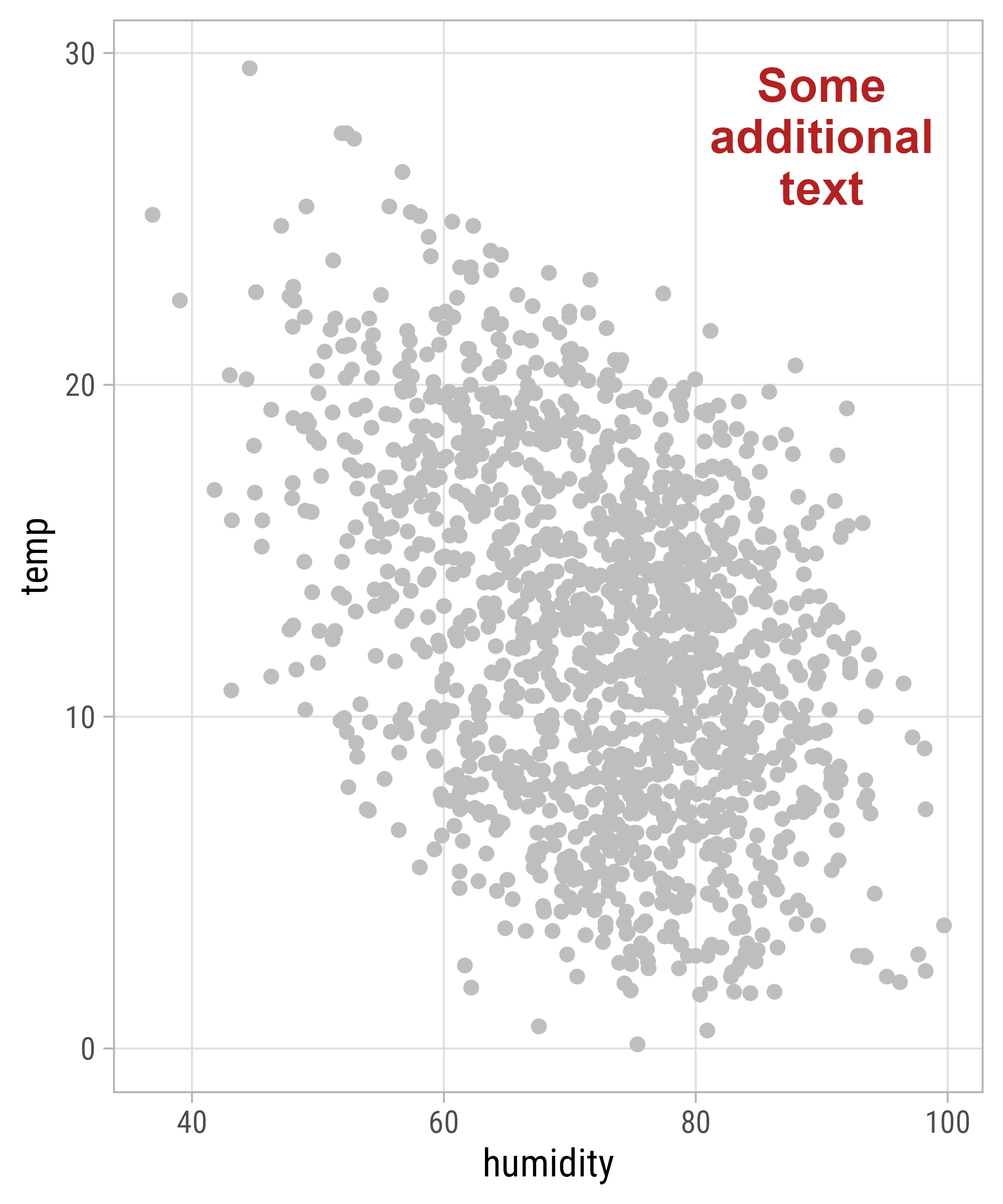
Add Arrows
ggplot(bikes, aes(humidity, temp)) +
  geom_point(size = 2, color = "grey") +
  annotate(
    geom = "text",
    x = 90,
    y = 27.5,
    label = "Some\nadditional\ntext",
    size = 6,
    lineheight = .9
  ) +
  annotate(
    geom = "curve",
    x = 94, xend = 82,
    y = 26, yend = 18.5,
    curvature = -.8,
    angle = 140,
    arrow = arrow(
      length = unit(10, "pt"),
      type = "closed"
    )
)![]()
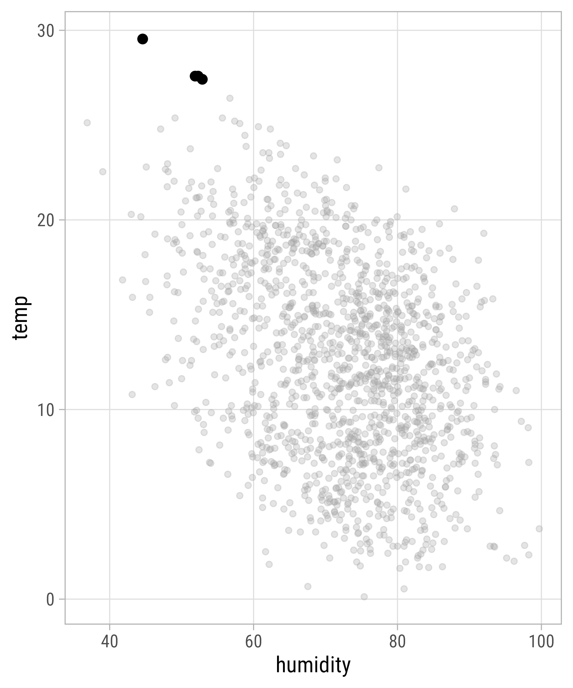
Highlight Hot Periods
Annotations with `geom_text()`
Annotations with `geom_label()`
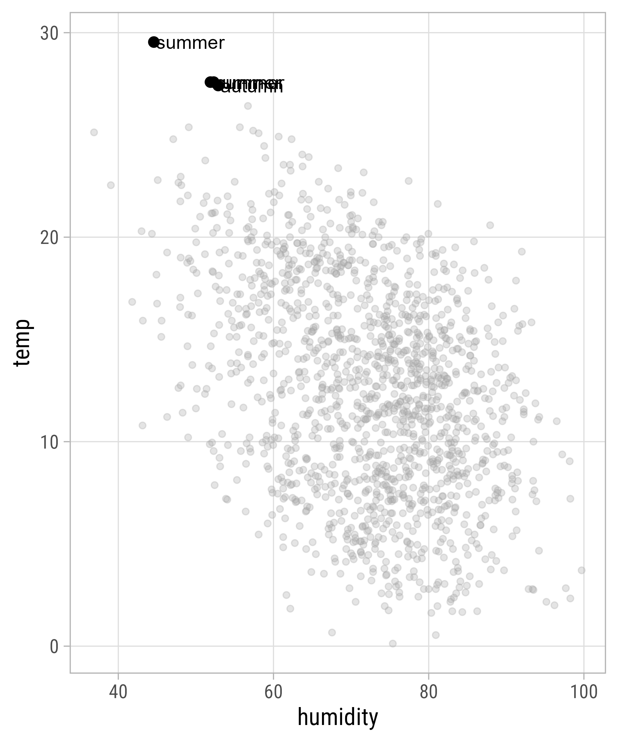
Annotations with {ggrepel}
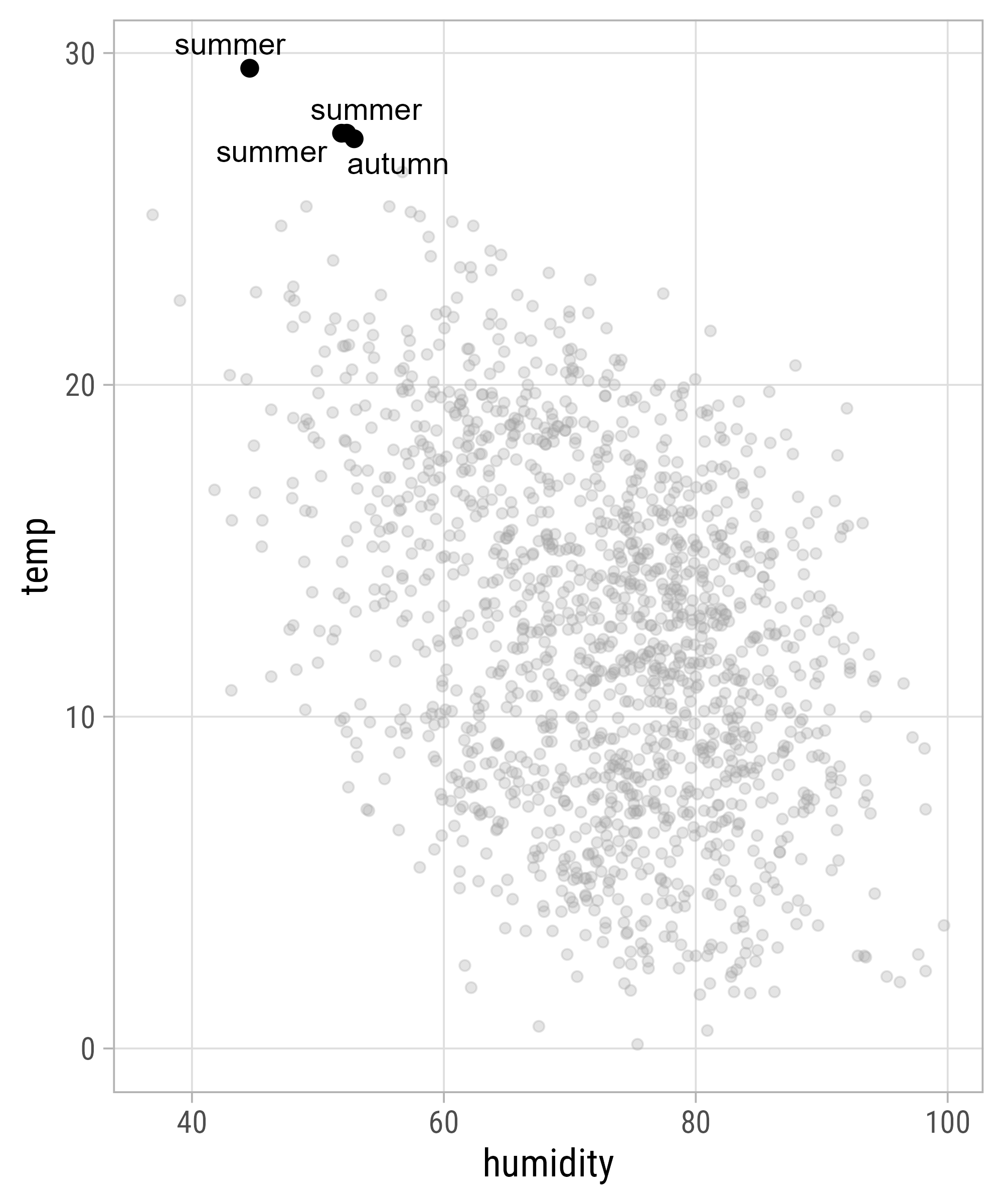
Annotations with {ggrepel}
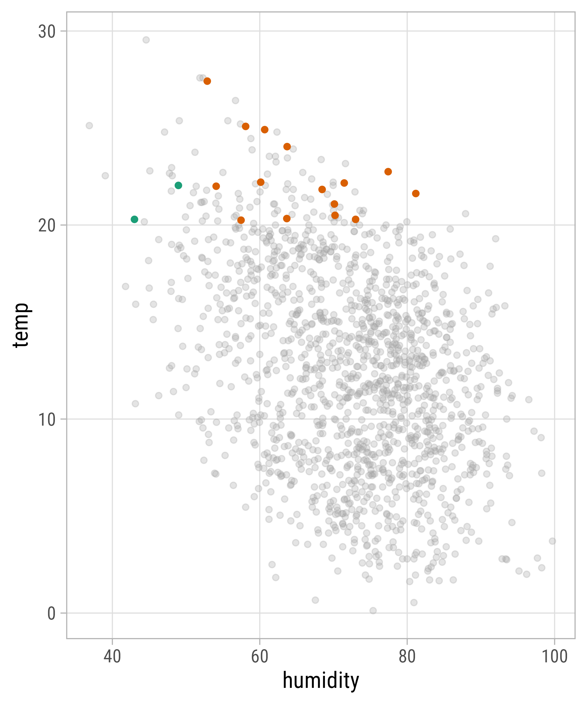
ggplot(
    filter(bikes, temp >= 27),
    aes(x = humidity, y = temp,
        color = season == "summer")
  ) +
  geom_point(
    data = bikes,
    color = "grey65", alpha = .3
  ) +
  geom_point(size = 2.5) +
  ggrepel::geom_text_repel(
    aes(label = str_to_title(season))
  ) +
  scale_color_manual(
    values = c("firebrick", "black"),
    guide = "none"
  )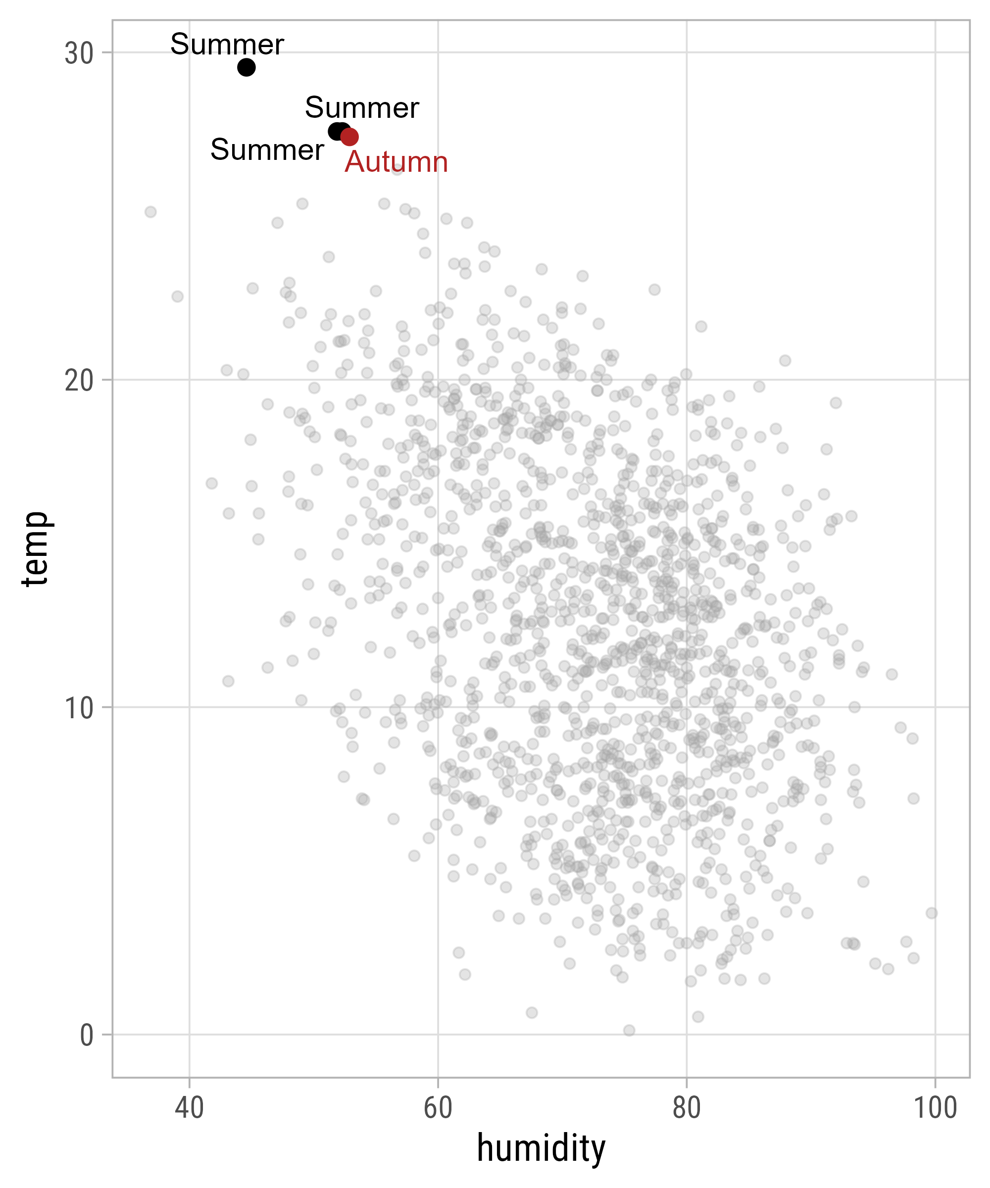
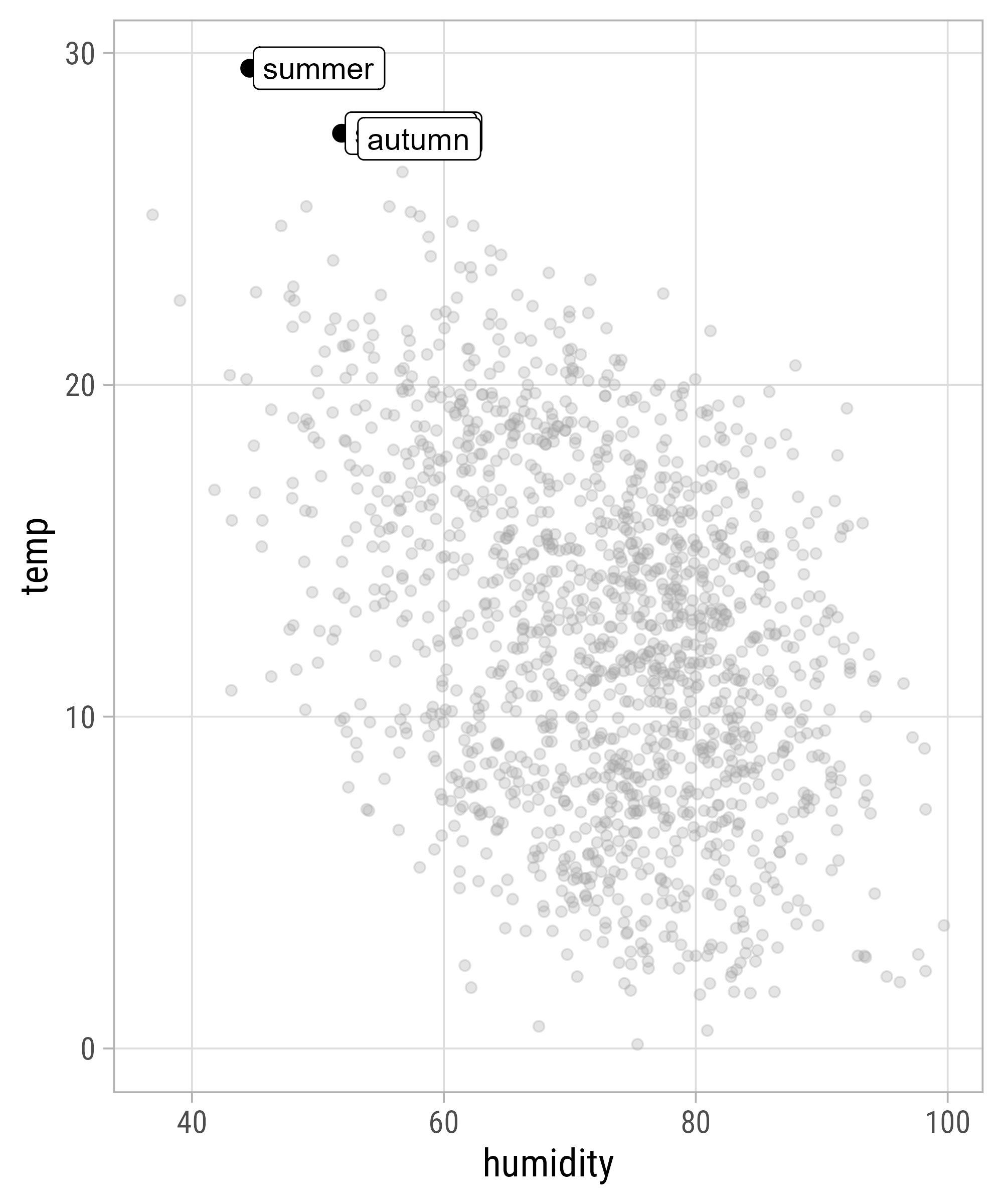
Annotations with {ggrepel}
ggplot(
    filter(bikes, temp >= 27),
    aes(x = humidity, y = temp,
        color = season == "summer")
  ) +
  geom_point(
    data = bikes,
    color = "grey65", alpha = .3
  ) +
  geom_point(size = 2.5) +
  ggrepel::geom_text_repel(
    aes(label = str_to_title(season)),
    ## space between points + labels
    box.padding = .4,
    ## always draw segments
    min.segment.length = 0
  ) +
  scale_color_manual(
    values = c("firebrick", "black"),
    guide = "none"
  )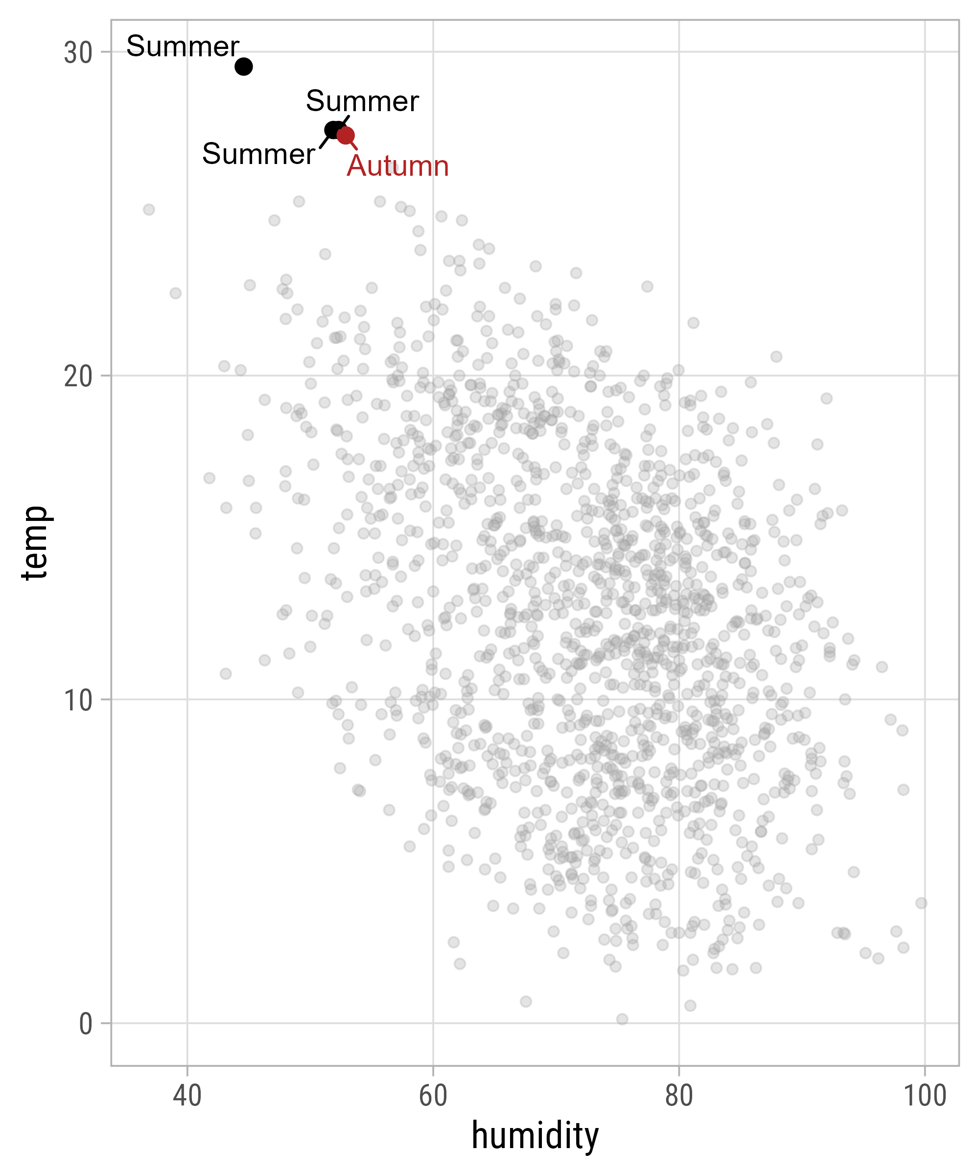
Annotations with {ggrepel}
ggplot(
    filter(bikes, temp >= 27),
    aes(x = humidity, y = temp,
        color = season == "summer")
  ) +
  geom_point(
    data = bikes,
    color = "grey65", alpha = .3
  ) +
  geom_point(size = 2.5) +
  ggrepel::geom_text_repel(
    aes(label = str_to_title(season)),
    ## force to the right
    xlim = c(NA, 35), hjust = 1
  ) +
  scale_color_manual(
    values = c("firebrick", "black"),
    guide = "none"
  ) +
  xlim(25, NA)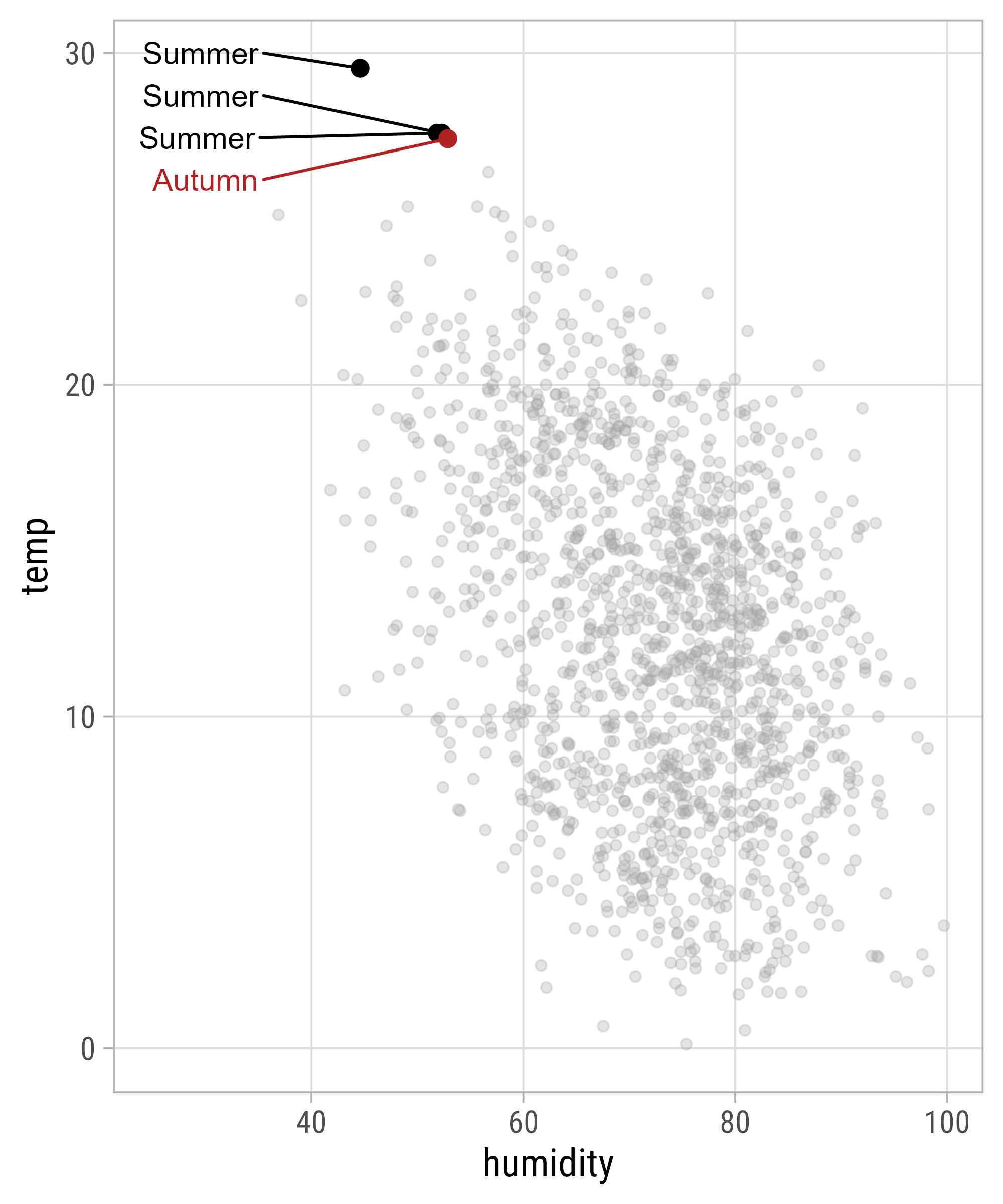
Annotations with {ggrepel}
ggplot(
    filter(bikes, temp >= 27),
    aes(x = humidity, y = temp,
        color = season == "summer")
  ) +
  geom_point(
    data = bikes,
    color = "grey65", alpha = .3
  ) +
  geom_point(size = 2.5) +
  ggrepel::geom_text_repel(
    aes(label = str_to_title(season)),
    ## force to the right
    xlim = c(NA, 35),
    ## style segment
    segment.curvature = .01,
    arrow = arrow(length = unit(.02, "npc"), type = "closed")
  ) +
  scale_color_manual(
    values = c("firebrick", "black"),
    guide = "none"
  ) +
xlim(25, NA)![]()
Annotations with {ggrepel}
ggplot(
    filter(bikes, temp >= 27),
    aes(x = humidity, y = temp,
        color = season == "summer")
  ) +
  geom_point(
    data = bikes,
    color = "grey65", alpha = .3
  ) +
  geom_point(size = 2.5) +
  ggrepel::geom_text_repel(
    aes(label = str_to_title(season)),
    ## force to the right
    xlim = c(NA, 35),
    ## style segment
    segment.curvature = .001,
    segment.inflect = TRUE
  ) +
  scale_color_manual(
    values = c("firebrick", "black"),
    guide = "none"
  ) +
  xlim(25, NA)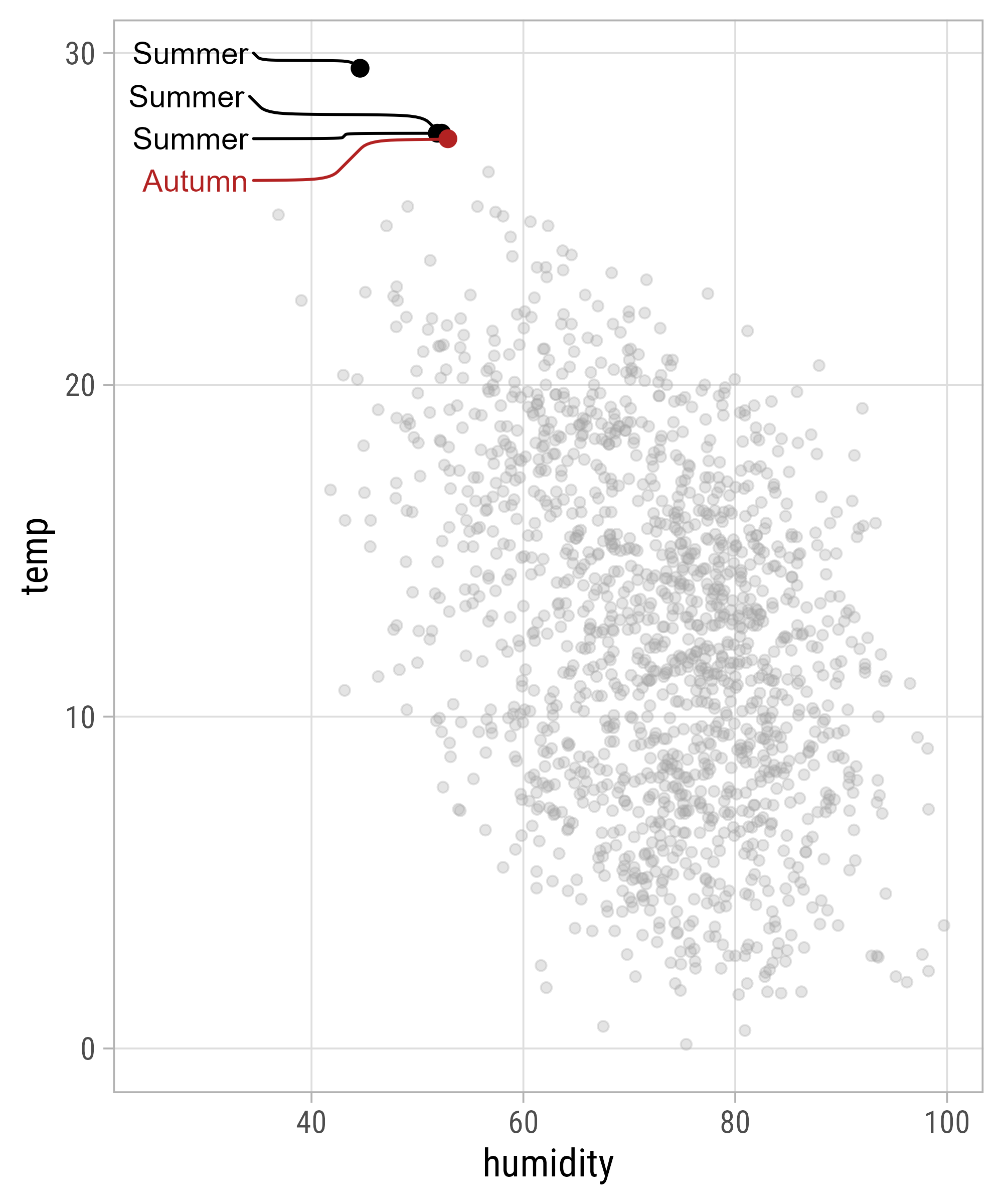
Annotations with {ggforce}
Annotations with {ggforce}
Annotations with {ggforce}
ggplot(
    filter(bikes, temp > 20 & season != "summer"),
    aes(x = humidity, y = temp,
        color = season)
  ) +
  geom_point(
    data = bikes,
    color = "grey65", alpha = .3
  ) +
  geom_point() +
  ggforce::geom_mark_rect(
    aes(label = str_to_title(season))
  ) +
  scale_color_brewer(
    palette = "Dark2",
    guide = "none"
) +
ylim(NA, 35)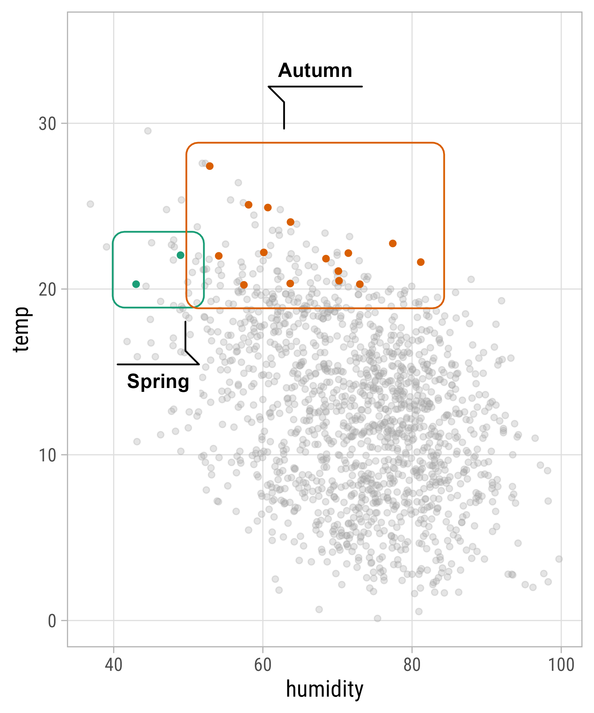
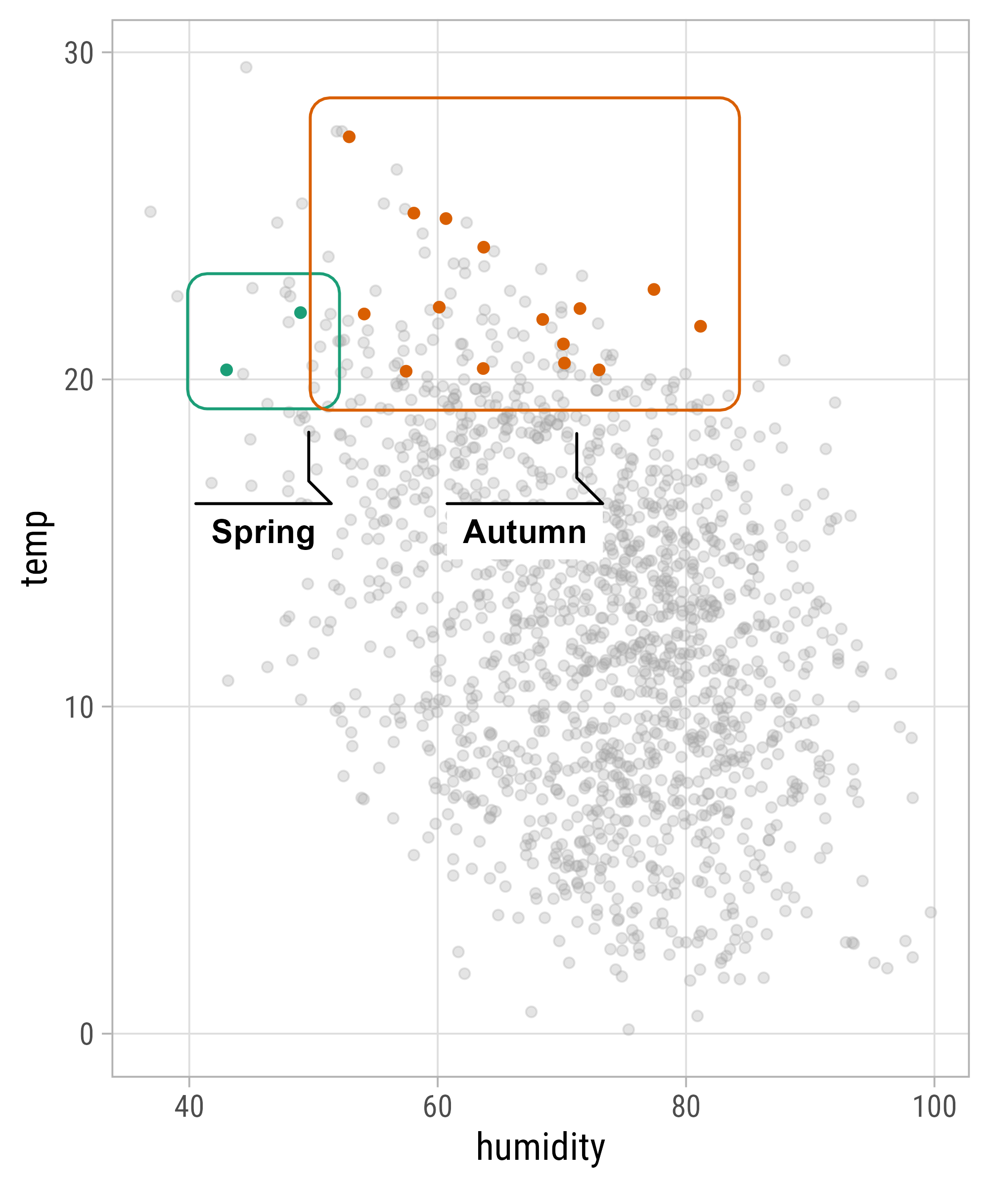
Annotations with {ggforce}
ggplot(
    filter(bikes, temp > 20 & season != "summer"),
    aes(x = humidity, y = temp,
        color = season)
  ) +
  geom_point(
    data = bikes,
    color = "grey65", alpha = .3
  ) +
  geom_point() +
  ggforce::geom_mark_rect(
    aes(label = str_to_title(season)),
    expand = unit(5, "pt"),
    radius = unit(0, "pt"),
    con.cap = unit(0, "pt"),
    label.buffer = unit(15, "pt"),
    con.type = "straight",
    label.fill = "transparent"
  ) +
  scale_color_brewer(
    palette = "Dark2",
    guide = "none"
  ) +
  ylim(NA, 35)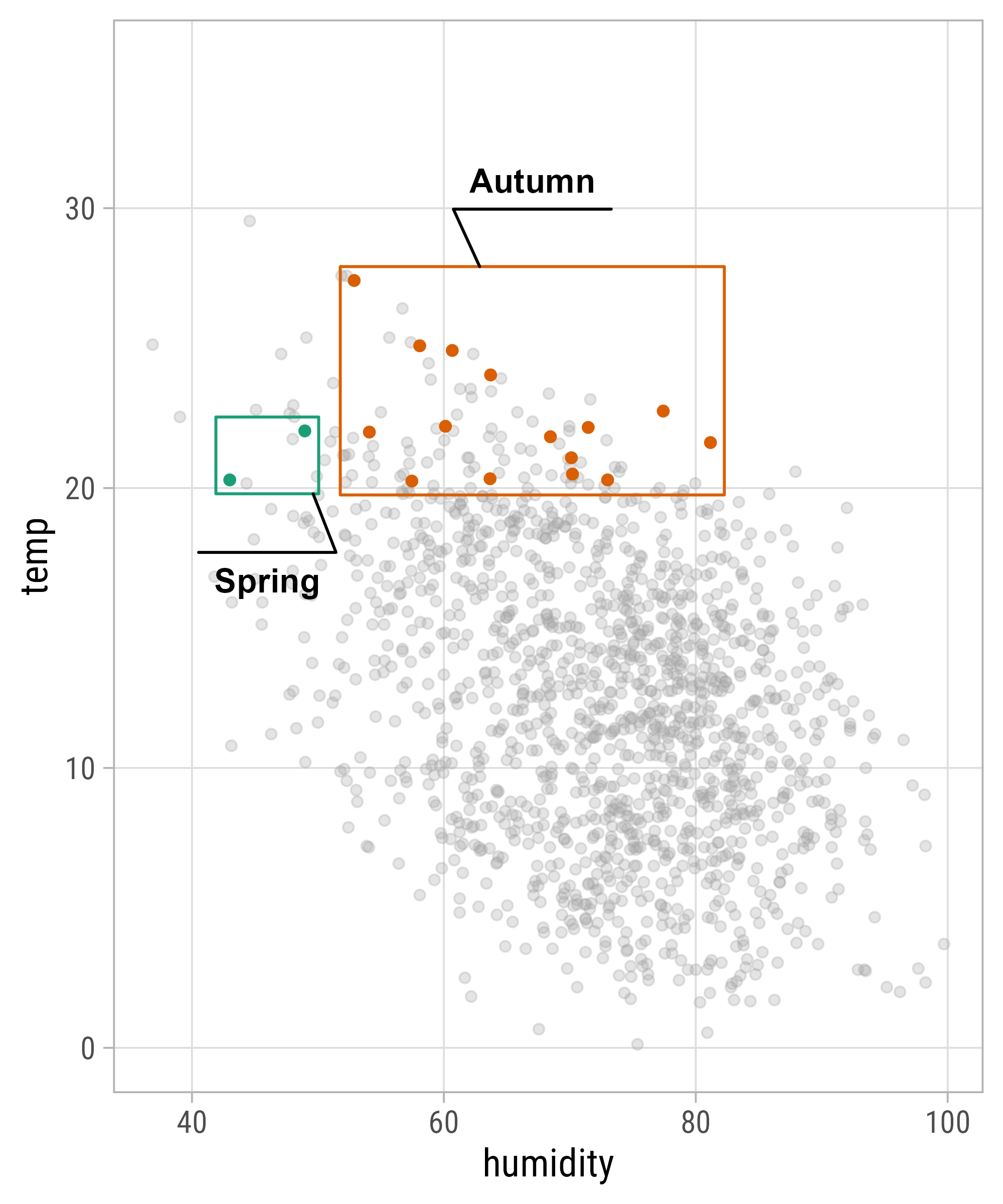
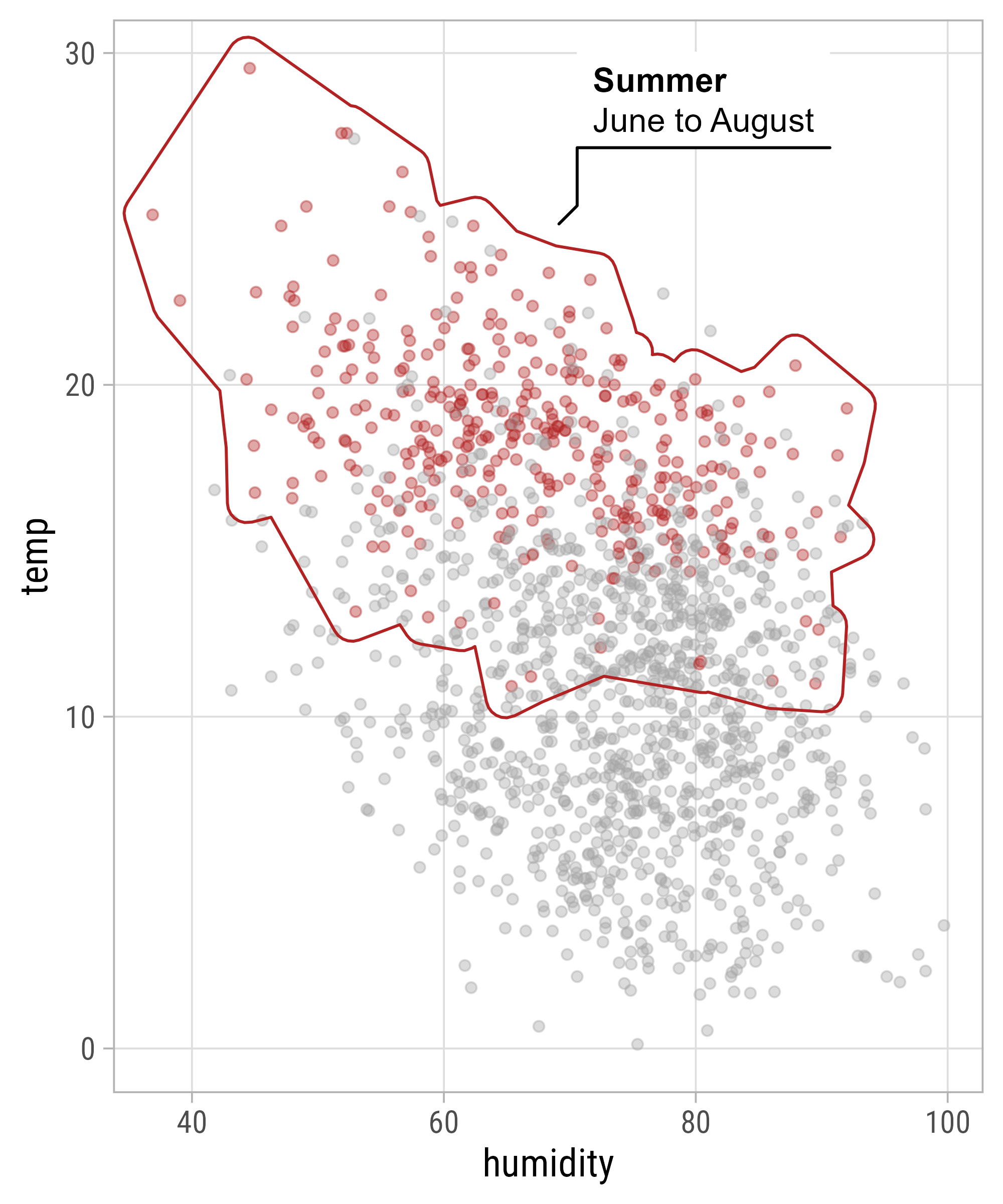
Annotations with {ggforce}
ggplot(
    bikes,
    aes(x = humidity, y = temp,
        color = season == "summer")
  ) +
  geom_point(alpha = .4) +
  ggforce::geom_mark_hull(
    aes(label = str_to_title(season),
        filter = season == "summer",
        description = "June to August"),
    expand = unit(10, "pt")
  ) +
  scale_color_manual(
    values = c("grey65", "firebrick"),
    guide = "none"
  )
Load and Modify Image

Add Background Image
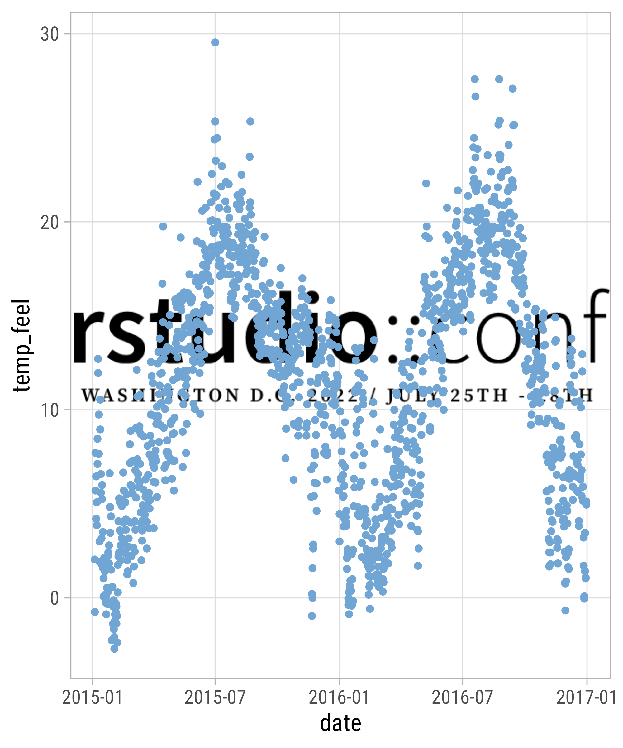
Adjust Position
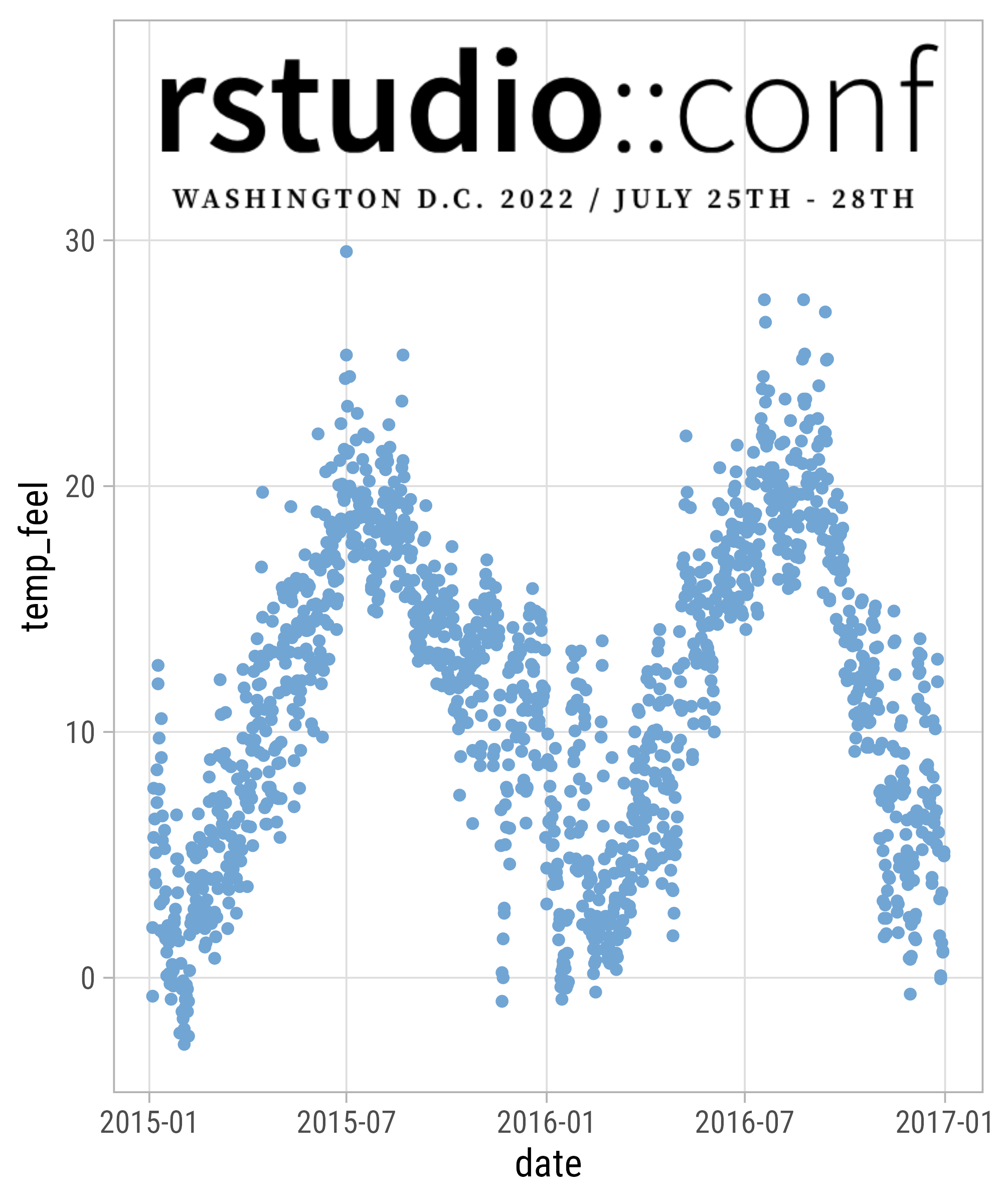
Place Image Outside
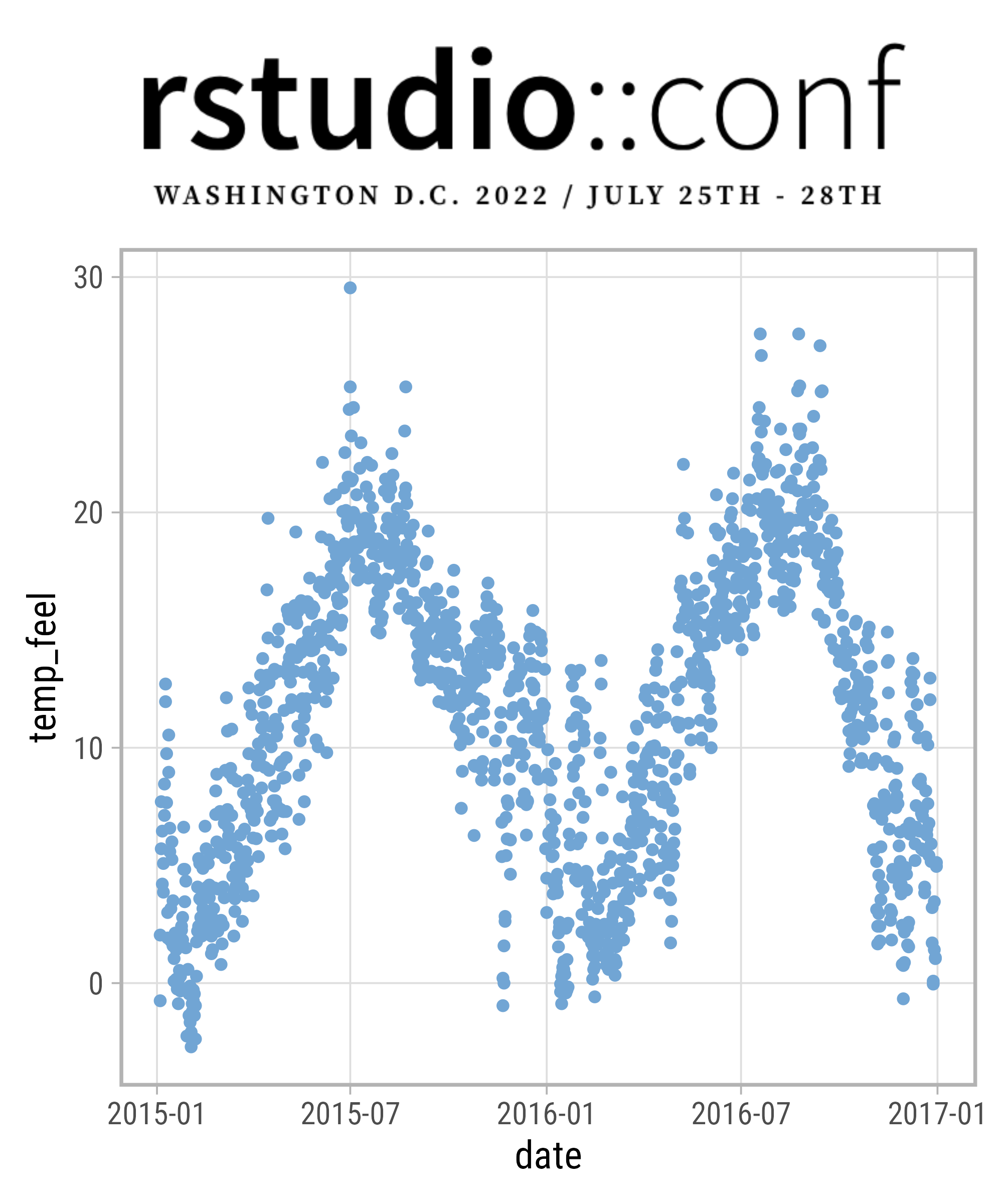
Exercise 2
- Create this logo with the image file
exercises/img/rstudioconf-washington-bg.pngfor the skyline: