library(tidyverse)

bikes <- readr::read_csv(
  here::here("data", "london-bikes-custom.csv"),
  col_types = "Dcfffilllddddc"
)

bikes$season <- forcats::fct_inorder(bikes$season)

theme_set(theme_light(base_size = 14, base_family = "Roboto Condensed"))

theme_update(
  panel.grid.minor = element_blank(),
  plot.title = element_text(face = "bold"),
  plot.title.position = "plot"
)Graphic Design with ggplot2
Working with Layouts and Composition
Discrete Legend
Continuous Legend
Legend Position

Legend Justification
Legend Position
Legend Direction

Legend Types
Legend Types
Legend Types
Legend Types

Legend Styling
Legend Styling
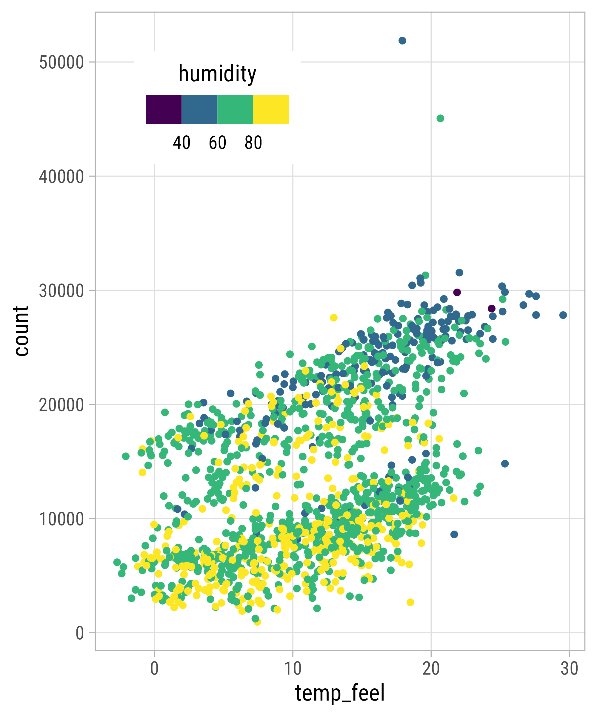
ggplot(
bikes,
aes(x = temp_feel, y = count,
color = humidity)
) +
geom_point() +
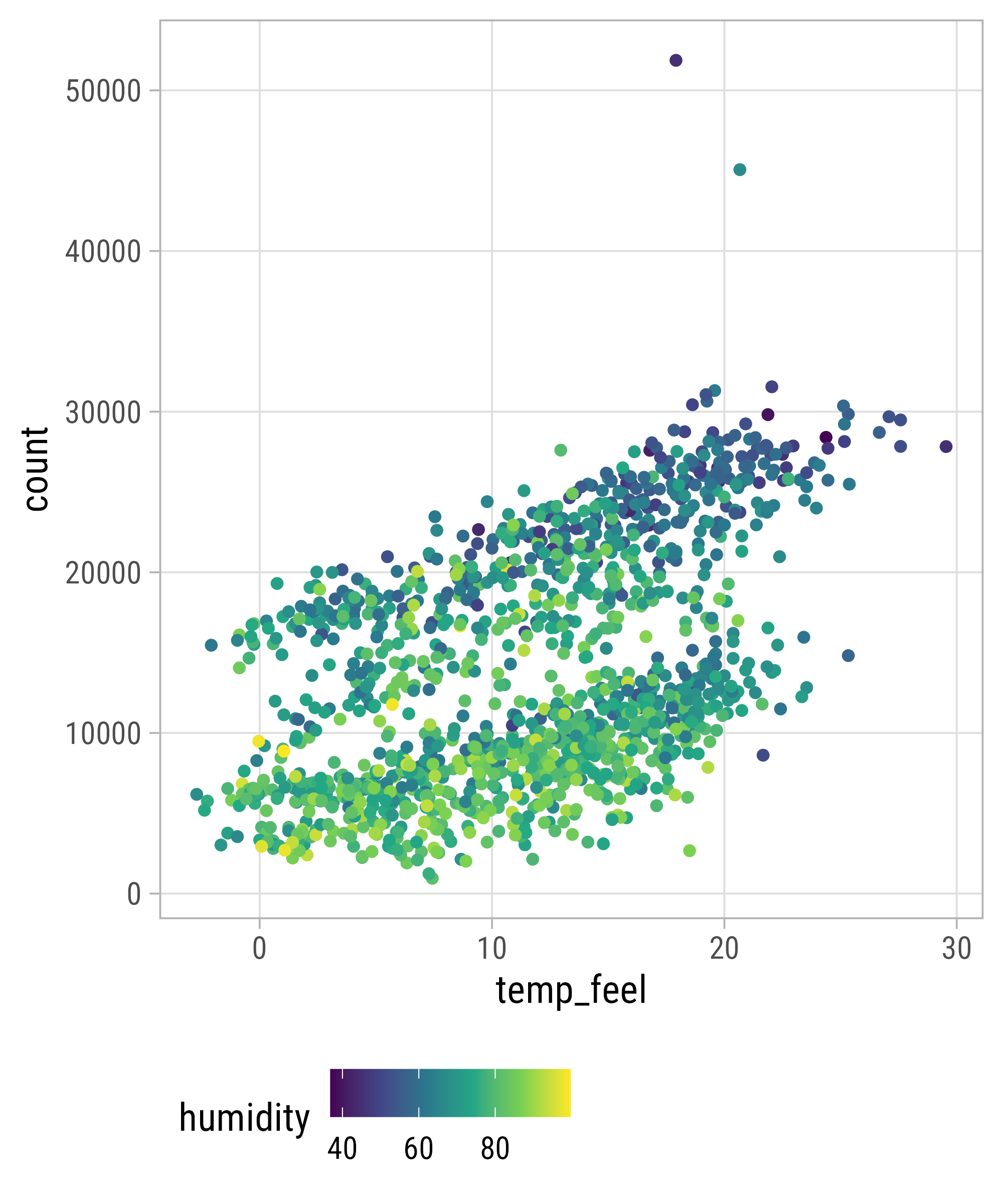
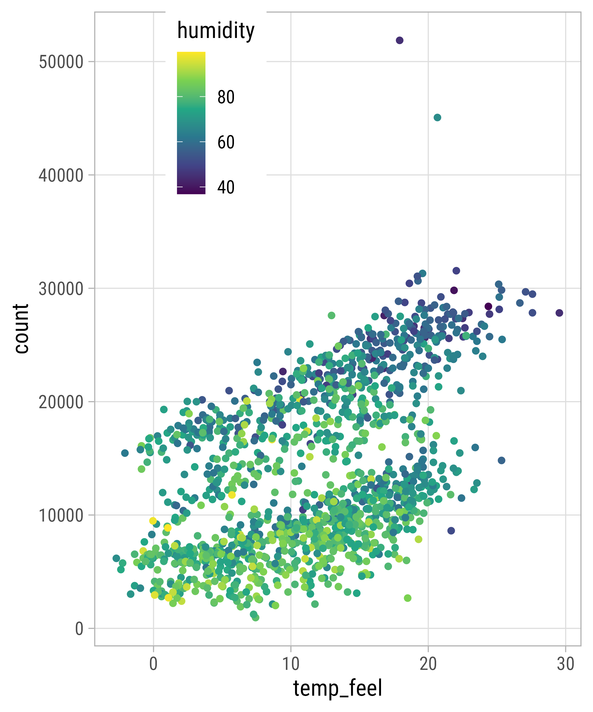
scale_color_viridis_b(
guide = guide_colorsteps(
title.position = "top",
title.hjust = .5,
show.limits = TRUE,
frame.colour = "black",
frame.linewidth = 3,
barwidth = unit(8, "lines")
)
) +
theme(
legend.position = c(.25, .85),
legend.direction = "horizontal"
)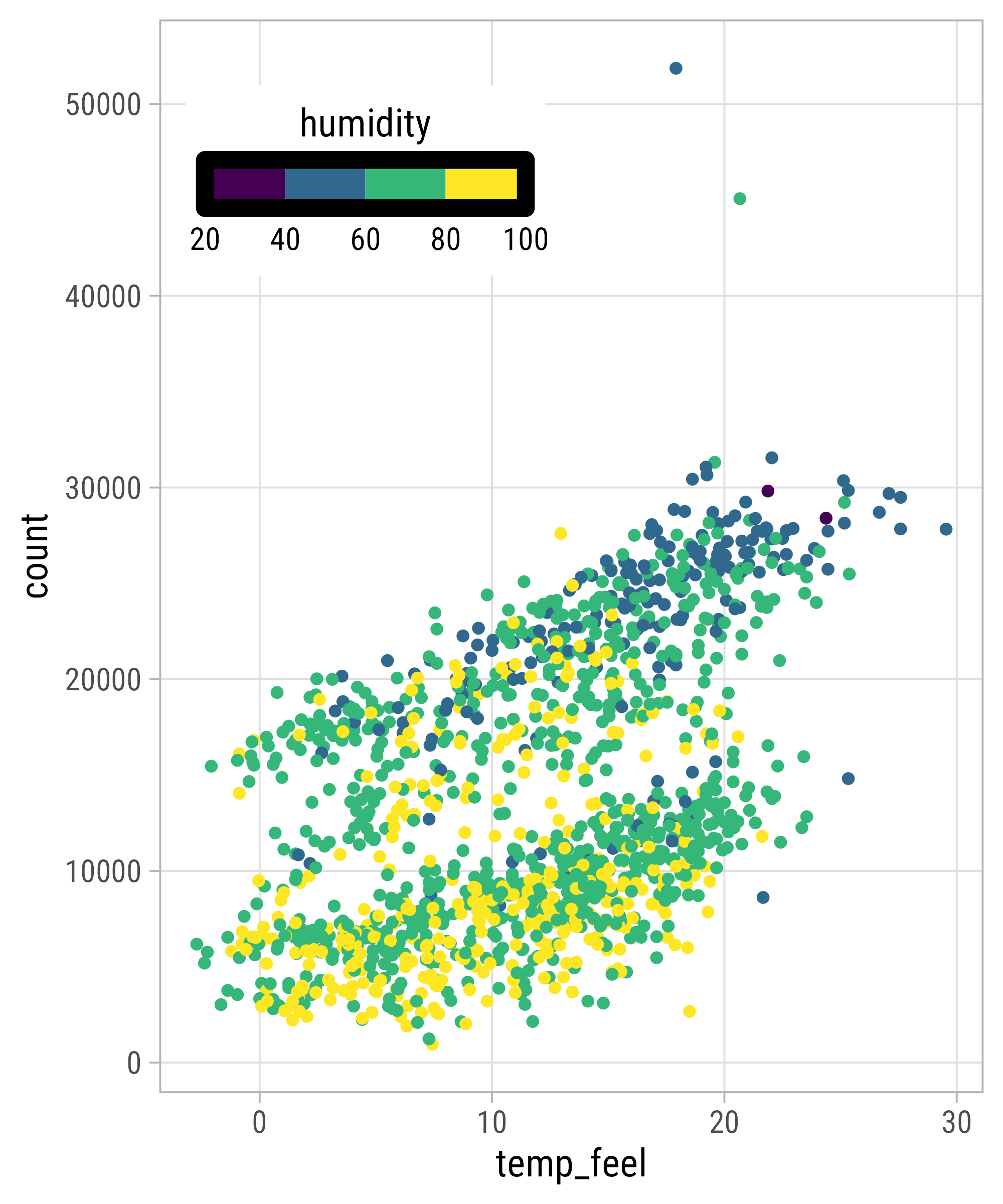
Legend Styling
ggplot(
bikes,
aes(x = temp_feel, y = count,
color = humidity)
) +
geom_point() +
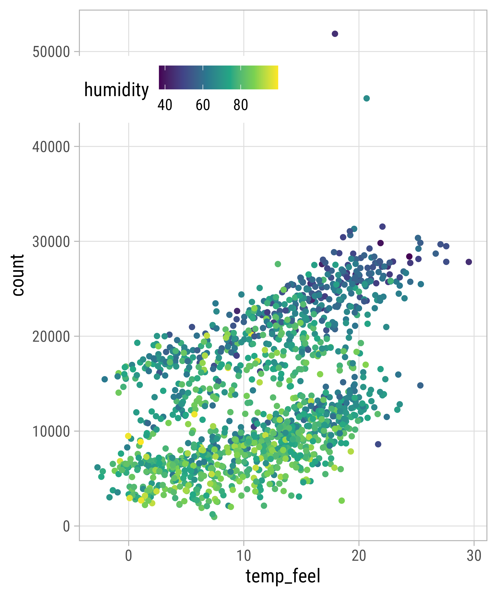
scale_color_viridis_c(
breaks = 3:10*10,
limits = c(30, 100),
guide = guide_colorbar(
title.position = "top",
title.hjust = .5,
ticks.linewidth = 3,
barwidth = unit(20, "lines"),
barheight = unit(.6, "lines")
)
) +
theme(
legend.position = "top"
)
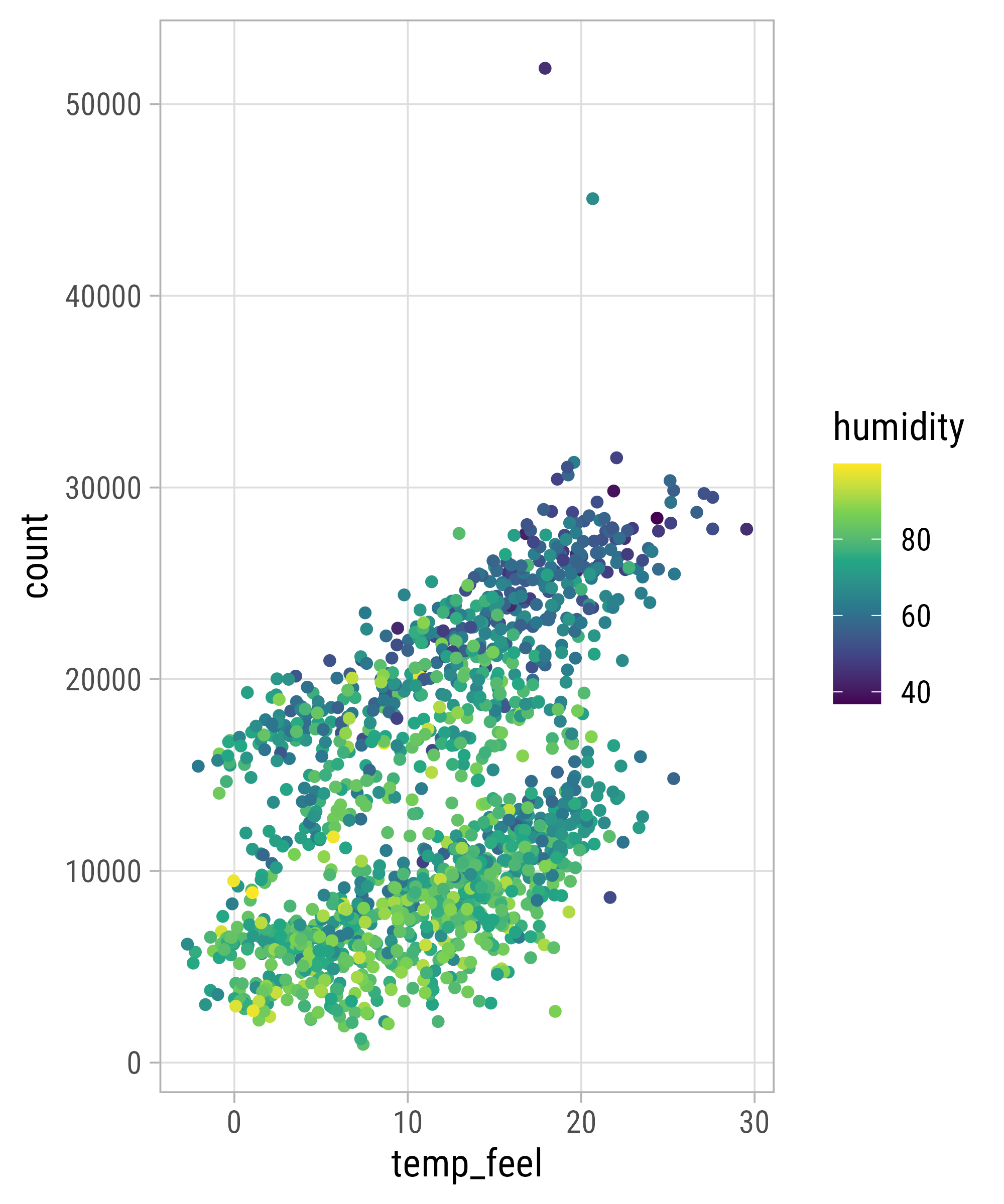
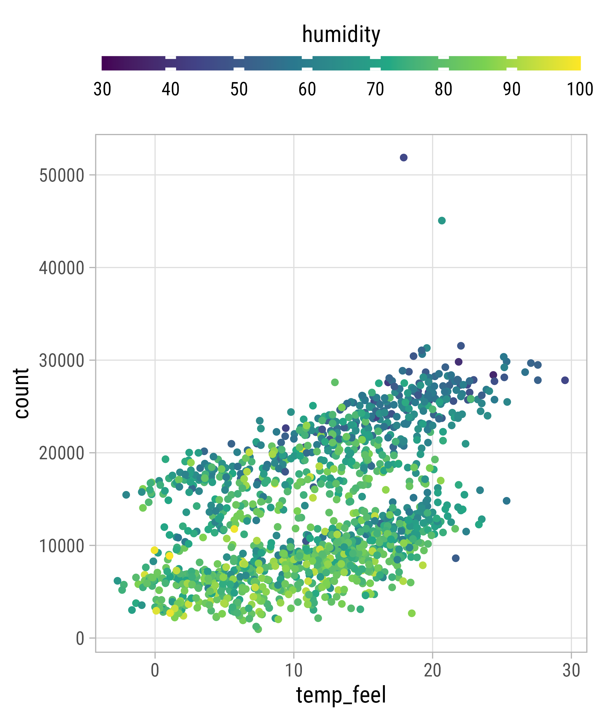
Legend Styling
ggplot(
bikes,
aes(x = temp_feel, y = count,
color = humidity)
) +
geom_point() +
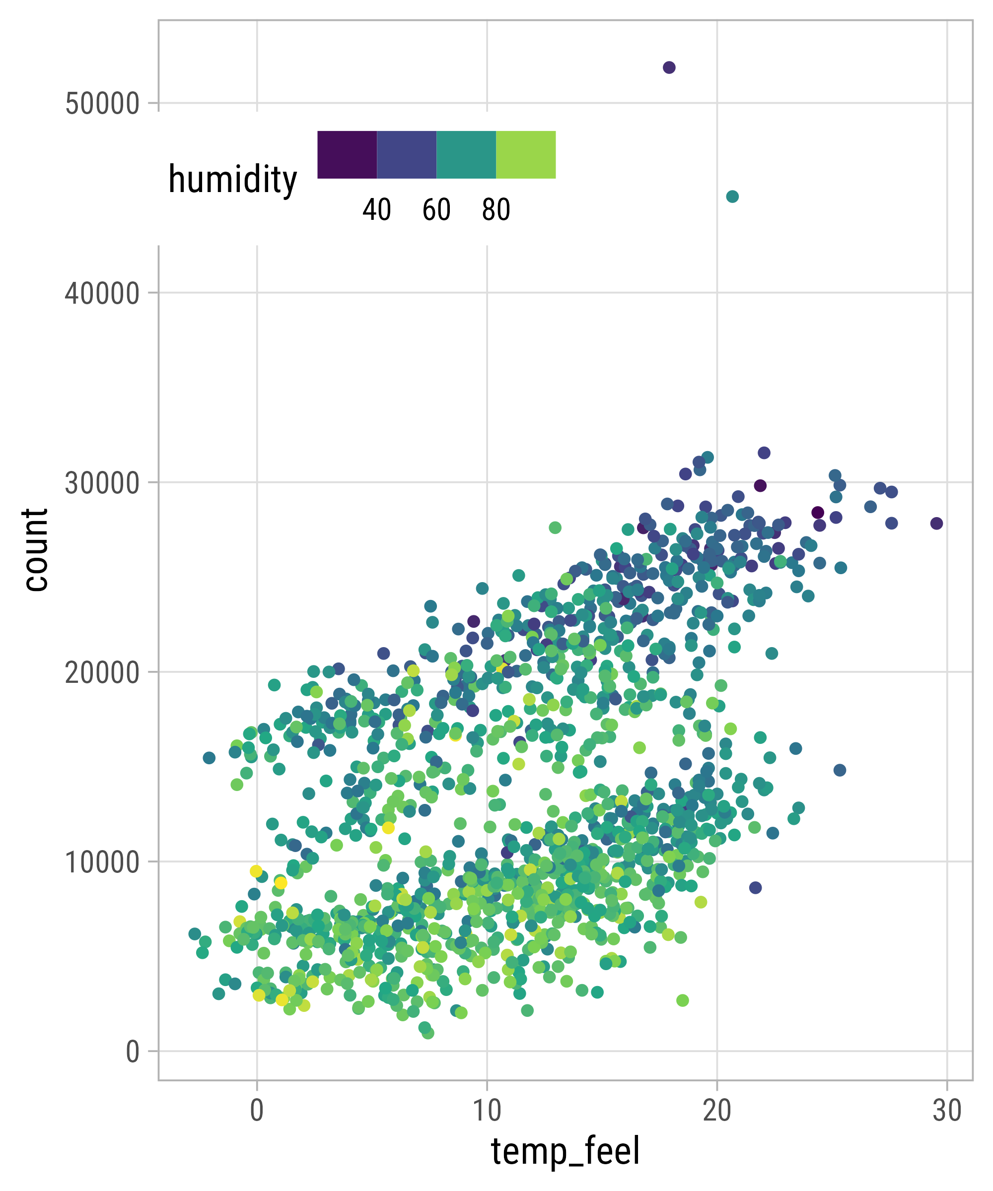
scale_color_viridis_c(
breaks = 3:10*10,
limits = c(30, 100),
guide = guide_colorbar(
title.position = "top",
title.hjust = .5,
ticks.linewidth = 3,
draw.ulim = FALSE,
draw.llim = FALSE,
barwidth = unit(20, "lines"),
barheight = unit(.6, "lines")
)
) +
theme(
legend.position = "top"
)
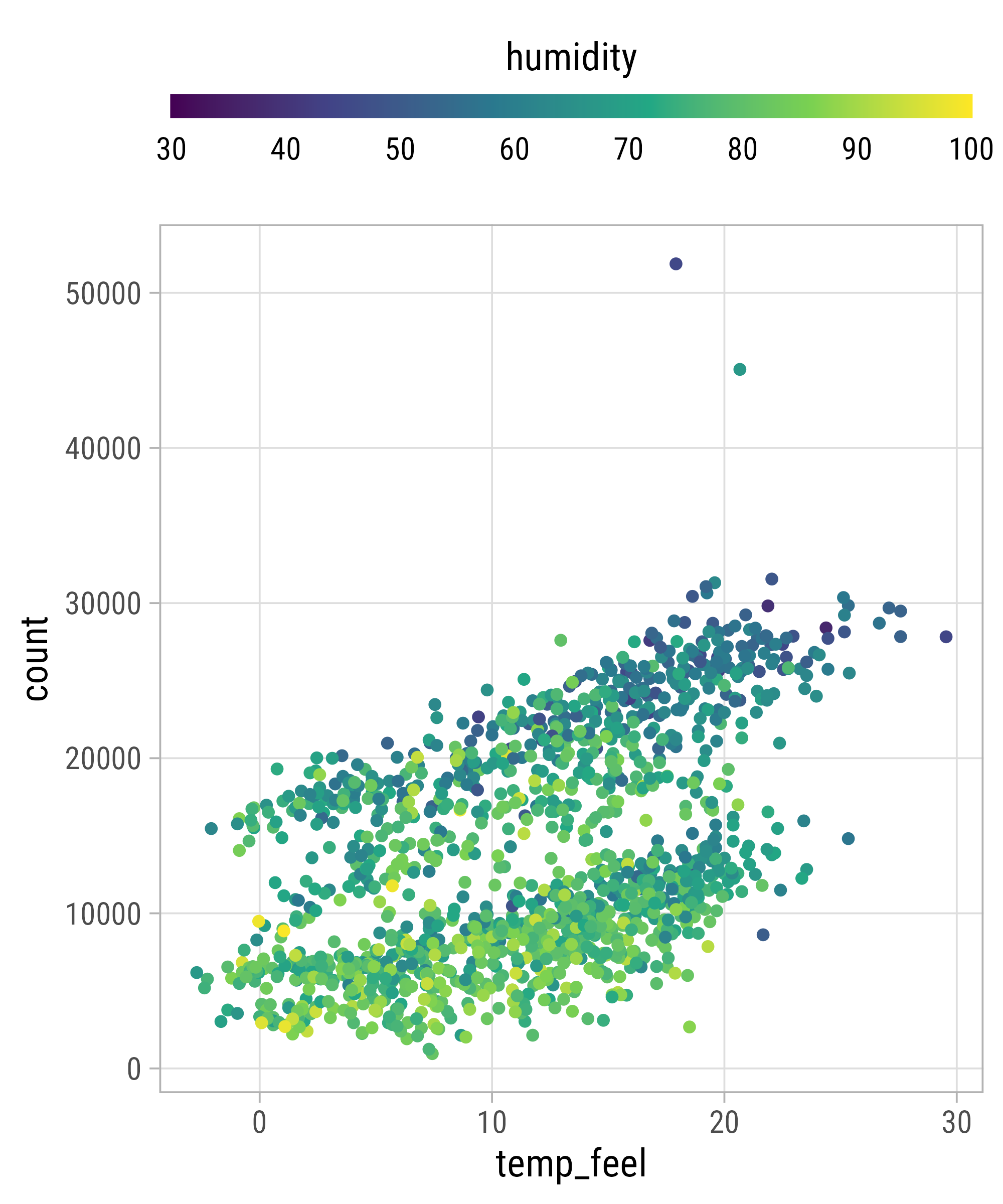
Legend Styling
ggplot(
bikes,
aes(x = temp_feel, y = count,
color = humidity)
) +
geom_point() +
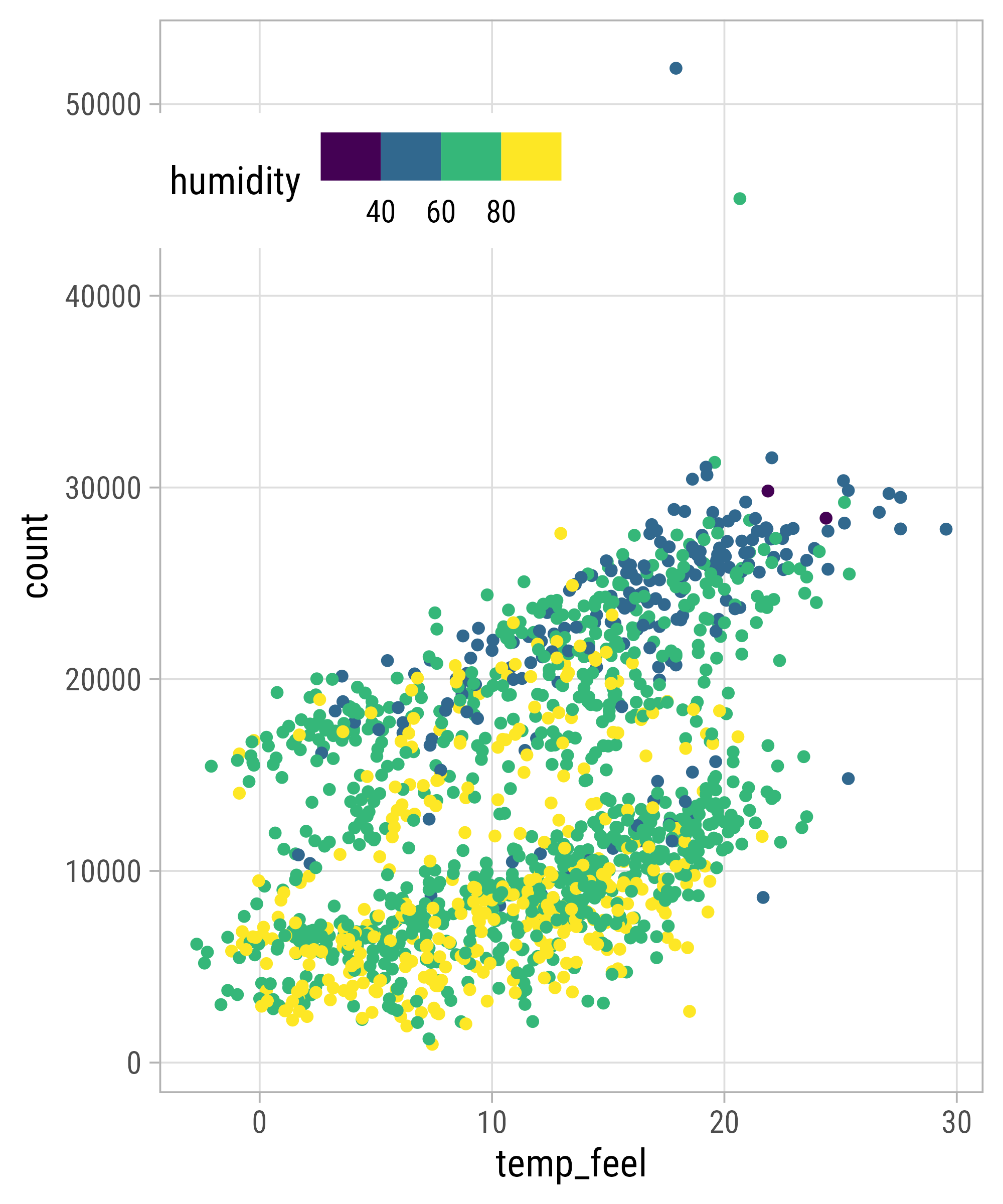
scale_color_viridis_c(
breaks = 3:10*10,
limits = c(30, 100),
guide = guide_colorbar(
title.position = "top",
title.hjust = .5,
ticks = FALSE,
barwidth = unit(20, "lines"),
barheight = unit(.6, "lines")
)
) +
theme(
legend.position = "top"
)
Key Glyphs
Key Glyphs
Key Glyphs

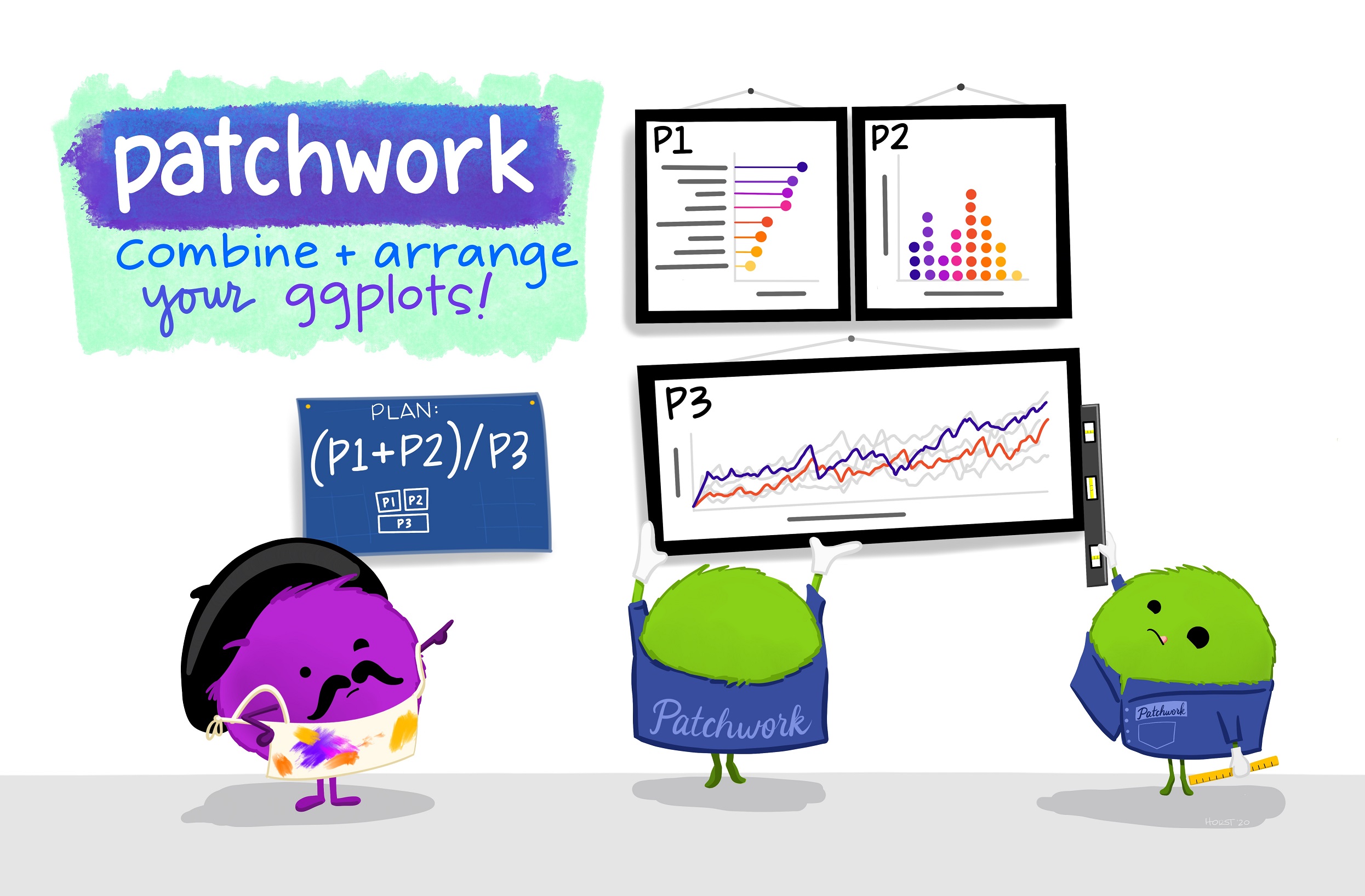
Illustration by Allison Horst
theme_std <- theme_set(theme_minimal(base_size = 18, base_family = "Pally"))
theme_update(
text = element_text(family = "Pally"),
panel.grid = element_blank(),
axis.text = element_text(color = "grey50", size = 12),
axis.title = element_text(color = "grey40", face = "bold"),
axis.title.x = element_text(margin = margin(t = 12)),
axis.title.y = element_text(margin = margin(r = 12)),
axis.line = element_line(color = "grey80", size = .4),
legend.text = element_text(color = "grey50", size = 12),
plot.tag = element_text(size = 40, margin = margin(b = 15)),
plot.background = element_rect(fill = "white", color = "white")
)
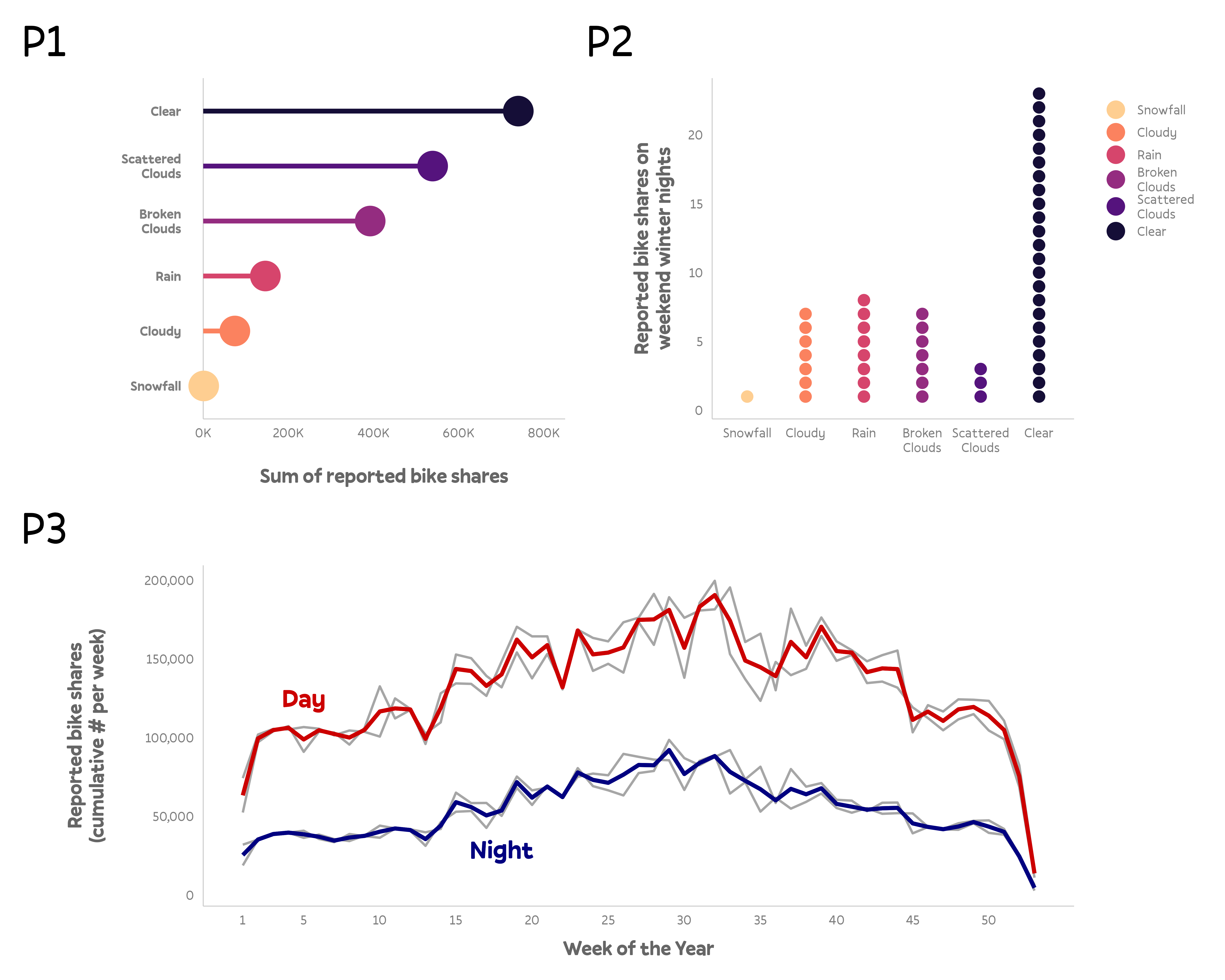
bikes_sorted <-
bikes %>%
filter(!is.na(weather_type)) %>%
group_by(weather_type) %>%
mutate(sum = sum(count)) %>%
ungroup() %>%
mutate(
weather_type = forcats::fct_reorder(
str_to_title(str_wrap(weather_type, 5)), sum
)
)
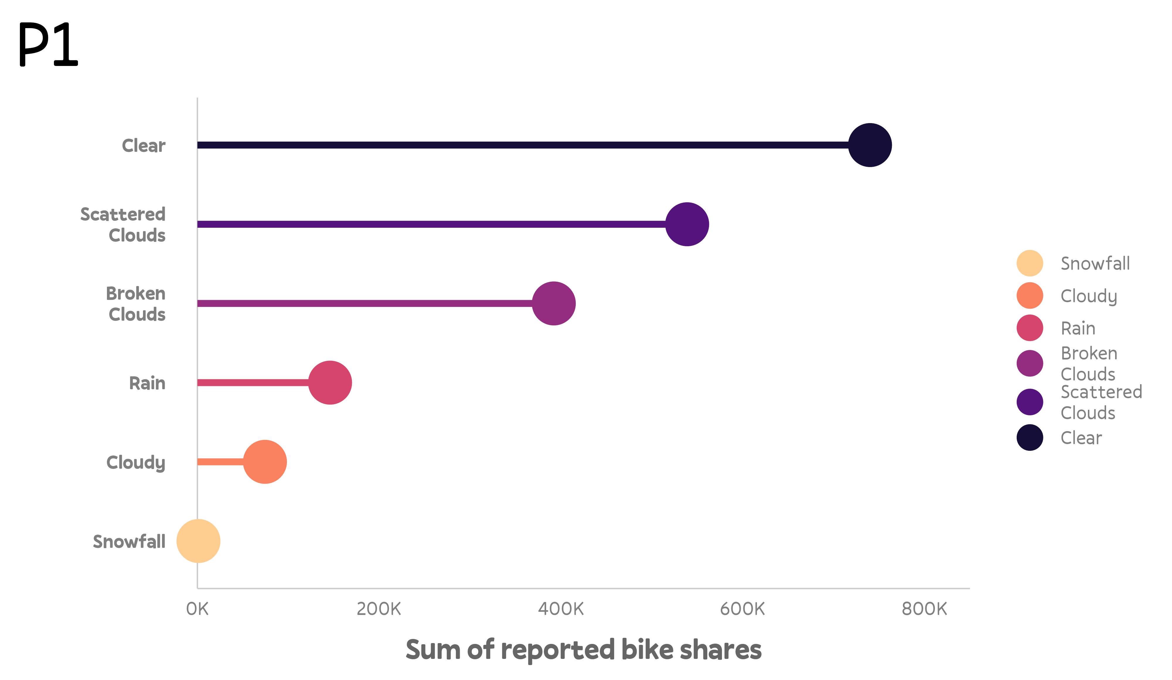
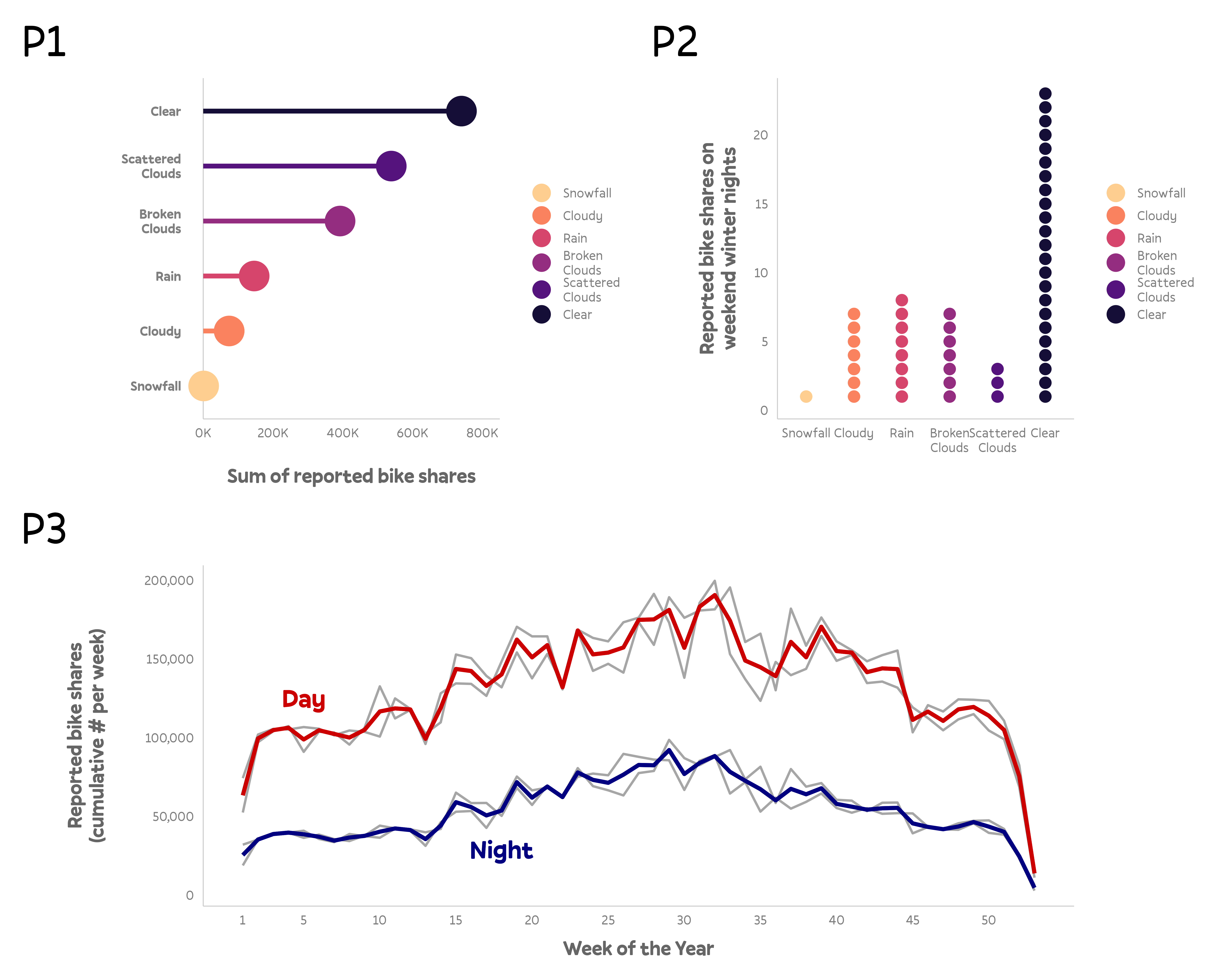
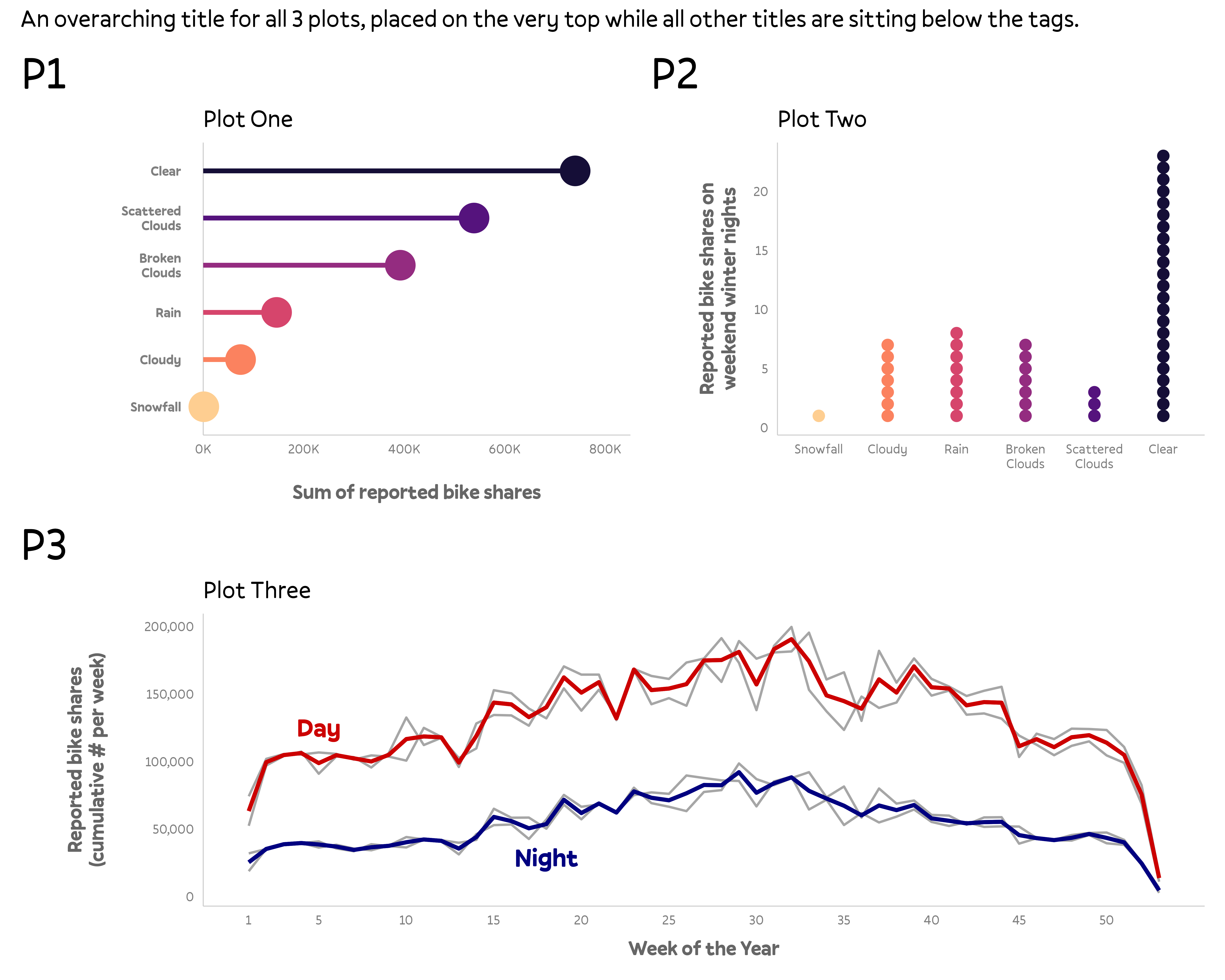
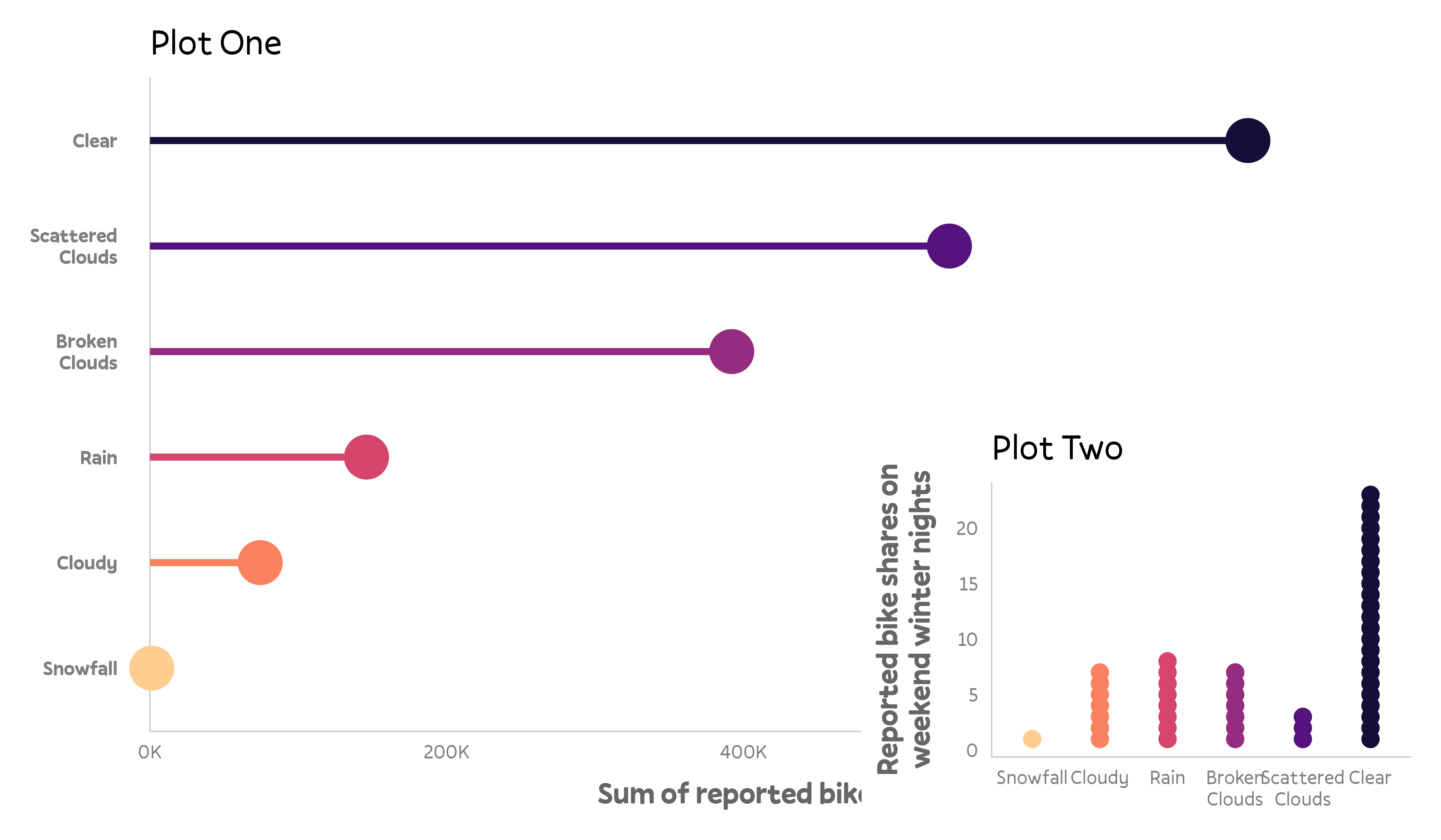
p1 <- ggplot(
bikes_sorted,
aes(x = weather_type, y = count, color = weather_type)
) +
geom_hline(yintercept = 0, color = "grey80", size = .4) +
stat_summary(
geom = "point", fun = "sum", size = 12
) +
stat_summary(
geom = "linerange", ymin = 0, fun.max = function(y) sum(y),
size = 2, show.legend = FALSE
) +
coord_flip(ylim = c(0, NA), clip = "off") +
scale_y_continuous(
expand = c(0, 0), limits = c(0, 8500000),
labels = scales::comma_format(scale = .0001, suffix = "K")
) +
scale_color_viridis_d(
option = "magma", direction = -1, begin = .1, end = .9, name = NULL,
guide = guide_legend(override.aes = list(size = 7))
) +
labs(
x = NULL, y = "Sum of reported bike shares", tag = "P1",
) +
theme(
axis.line.y = element_blank(),
axis.text.y = element_text(family = "Pally", color = "grey50", face = "bold",
margin = margin(r = 15), lineheight = .9)
)
p1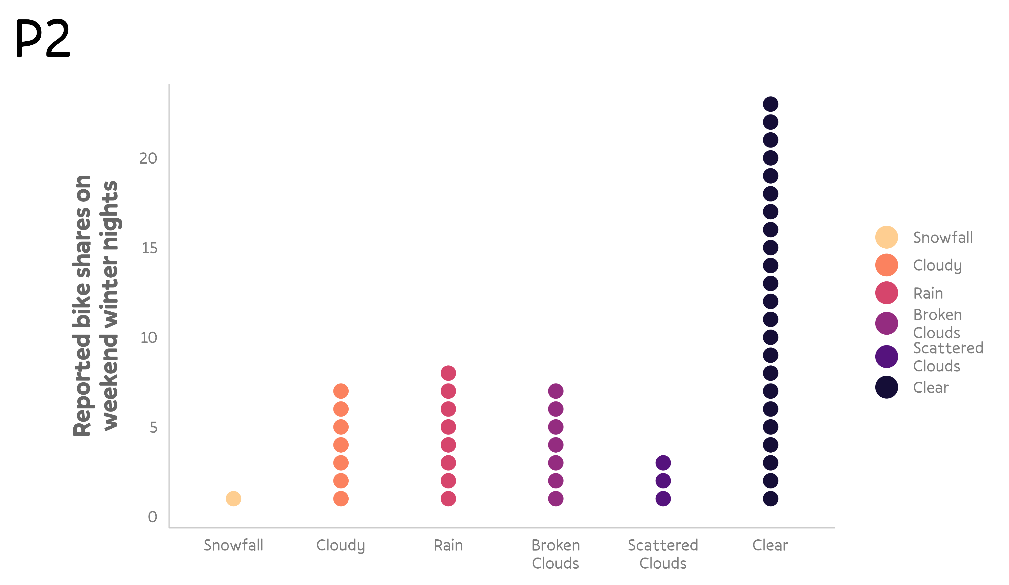
p2 <- bikes_sorted %>%
  filter(season == "winter", is_weekend == TRUE, day_night == "night") %>%
  group_by(weather_type, .drop = FALSE) %>%
  mutate(id = row_number()) %>%
  ggplot(
      aes(x = weather_type, y = id, color = weather_type)
    ) +
    geom_point(size = 4.5) +
    scale_color_viridis_d(
      option = "magma", direction = -1, begin = .1, end = .9, name = NULL,
      guide = guide_legend(override.aes = list(size = 7))
    ) +
    labs(
      x = NULL, y = "Reported bike shares on\nweekend winter nights", tag = "P2",
    ) +
    coord_cartesian(ylim = c(.5, NA), clip = "off")

p2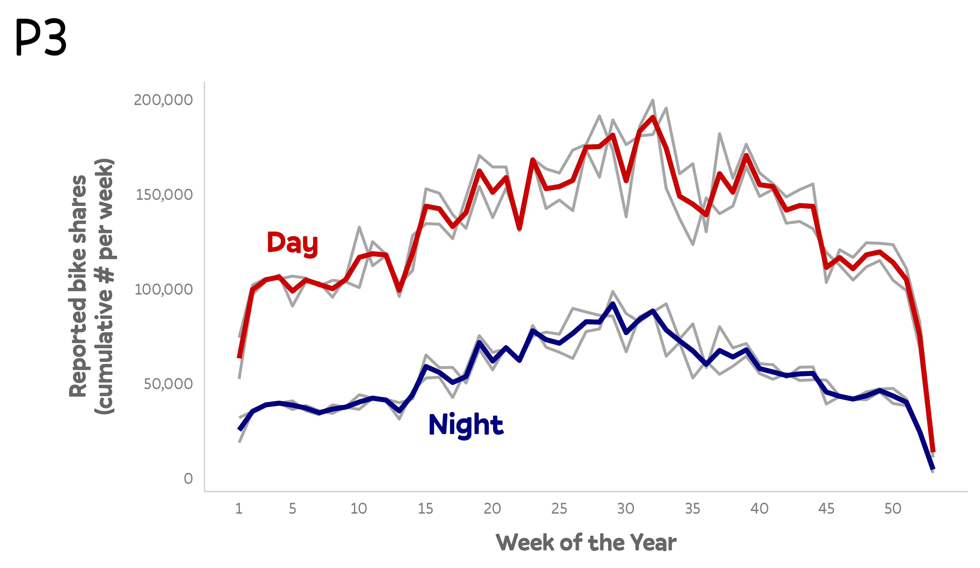
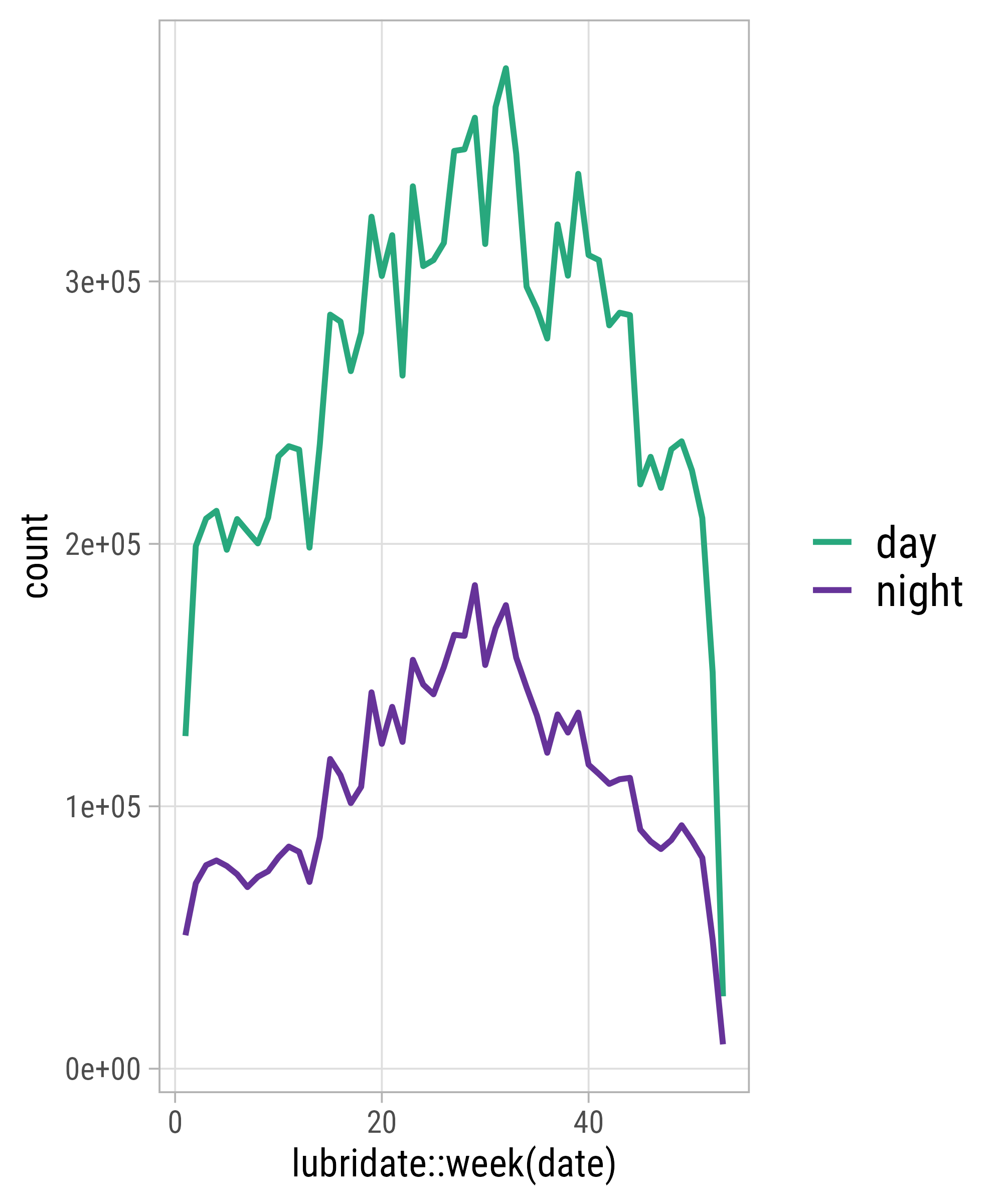
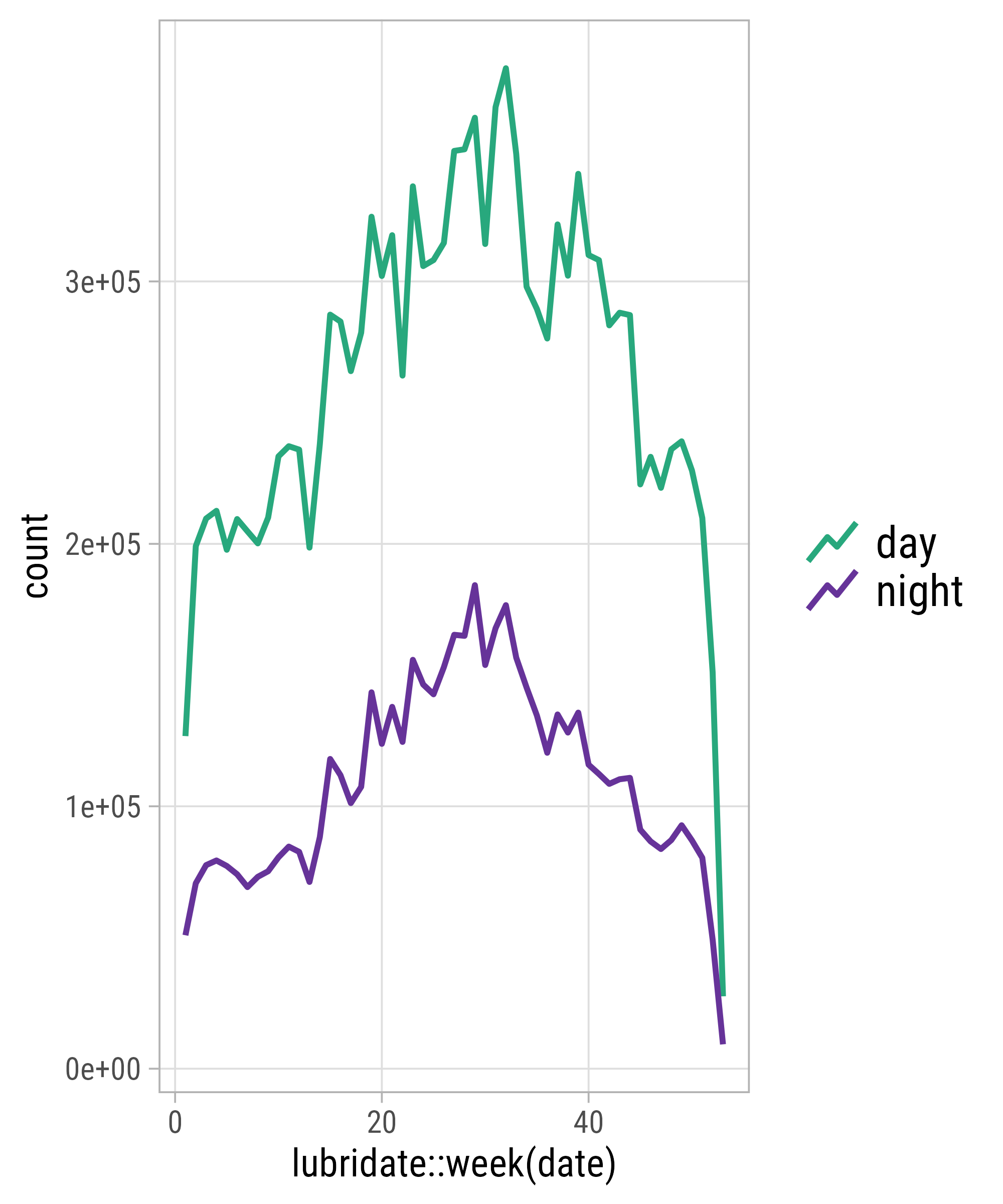
my_colors <- c("#cc0000", "#000080")
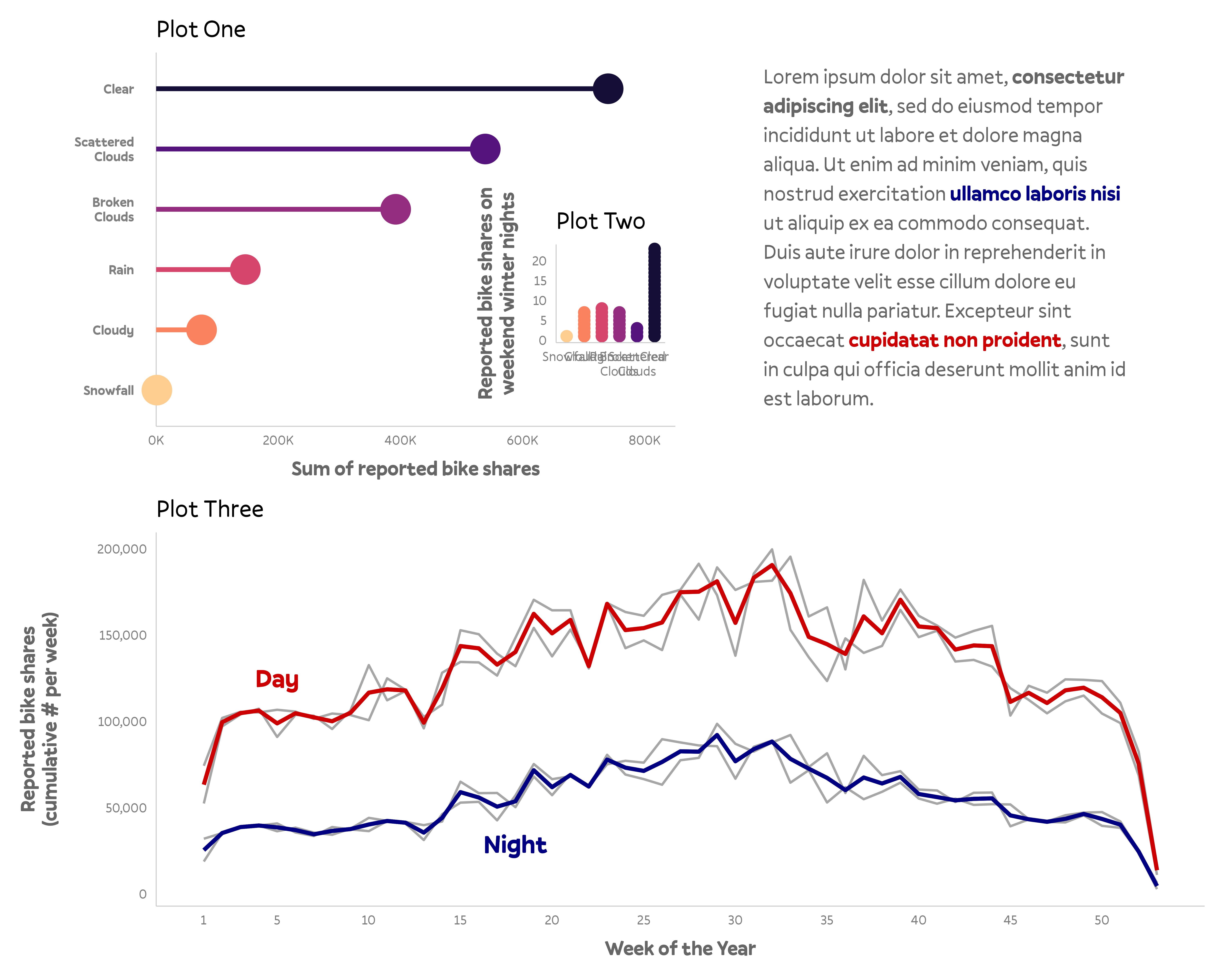
p3 <- bikes %>%
group_by(week = lubridate::week(date), day_night, year) %>%
summarize(count = sum(count)) %>%
group_by(week, day_night) %>%
mutate(avg = mean(count)) %>%
ggplot(aes(x = week, y = count, group = interaction(day_night, year))) +
geom_line(color = "grey65", size = 1) +
geom_line(aes(y = avg, color = day_night), stat = "unique", size = 1.7) +
annotate(
geom = "text", label = c("Day", "Night"), color = my_colors,
x = c(5, 18), y = c(125000, 29000), size = 8, fontface = "bold", family = "Pally"
) +
scale_x_continuous(breaks = c(1, 1:10*5)) +
scale_y_continuous(labels = scales::comma_format()) +
scale_color_manual(values = my_colors, guide = "none") +
labs(
x = "Week of the Year", y = "Reported bike shares\n(cumulative # per week)", tag = "P3",
)
p3{patchwork}
“Collect Guides”
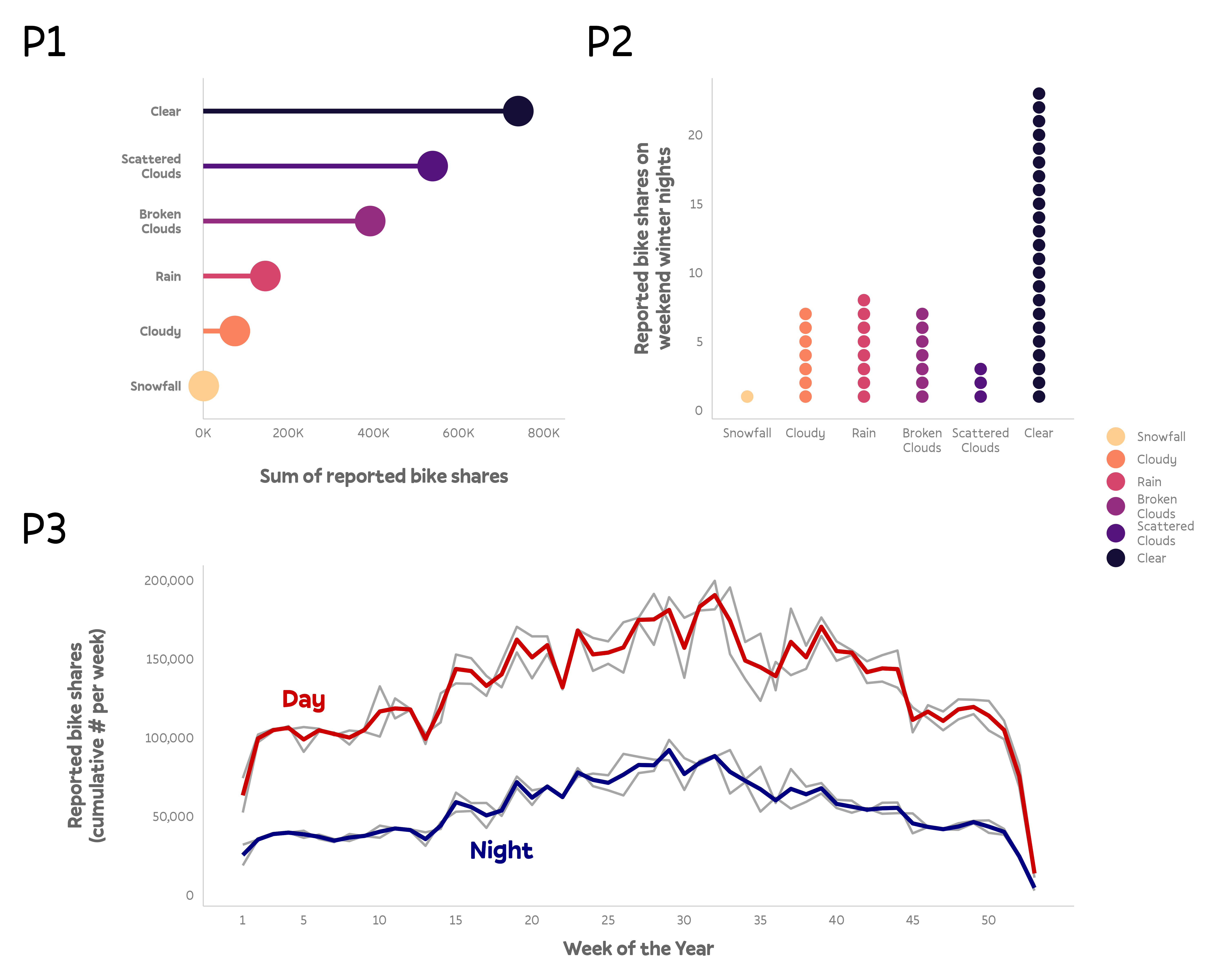
Apply Theming
Apply Theming
Adjust Widths and Heights
Use A Custom Layout
Add Labels
Add Text
text <- tibble(
  x = 0, y = 0, label = "Lorem ipsum dolor sit amet, **consectetur adipiscing elit**, sed do eiusmod tempor incididunt ut labore et dolore magna aliqua. Ut enim ad minim veniam, quis nostrud exercitation <b style='color:#000080;'>ullamco laboris nisi</b> ut aliquip ex ea commodo consequat. Duis aute irure dolor in reprehenderit in voluptate velit esse cillum dolore eu fugiat nulla pariatur. Excepteur sint occaecat <b style='color:#cc0000;'>cupidatat non proident</b>, sunt in culpa qui officia deserunt mollit anim id est laborum."
)

pt <- ggplot(text, aes(x = x, y = y)) +
  ggtext::geom_textbox(
    aes(label = label),
    box.color = NA, width = unit(23, "lines"),
    family = "Pally", color = "grey40", size = 6.5, lineheight = 1.4
  ) +
  coord_cartesian(expand = FALSE, clip = "off") +
  theme_void()

pt
Add Text
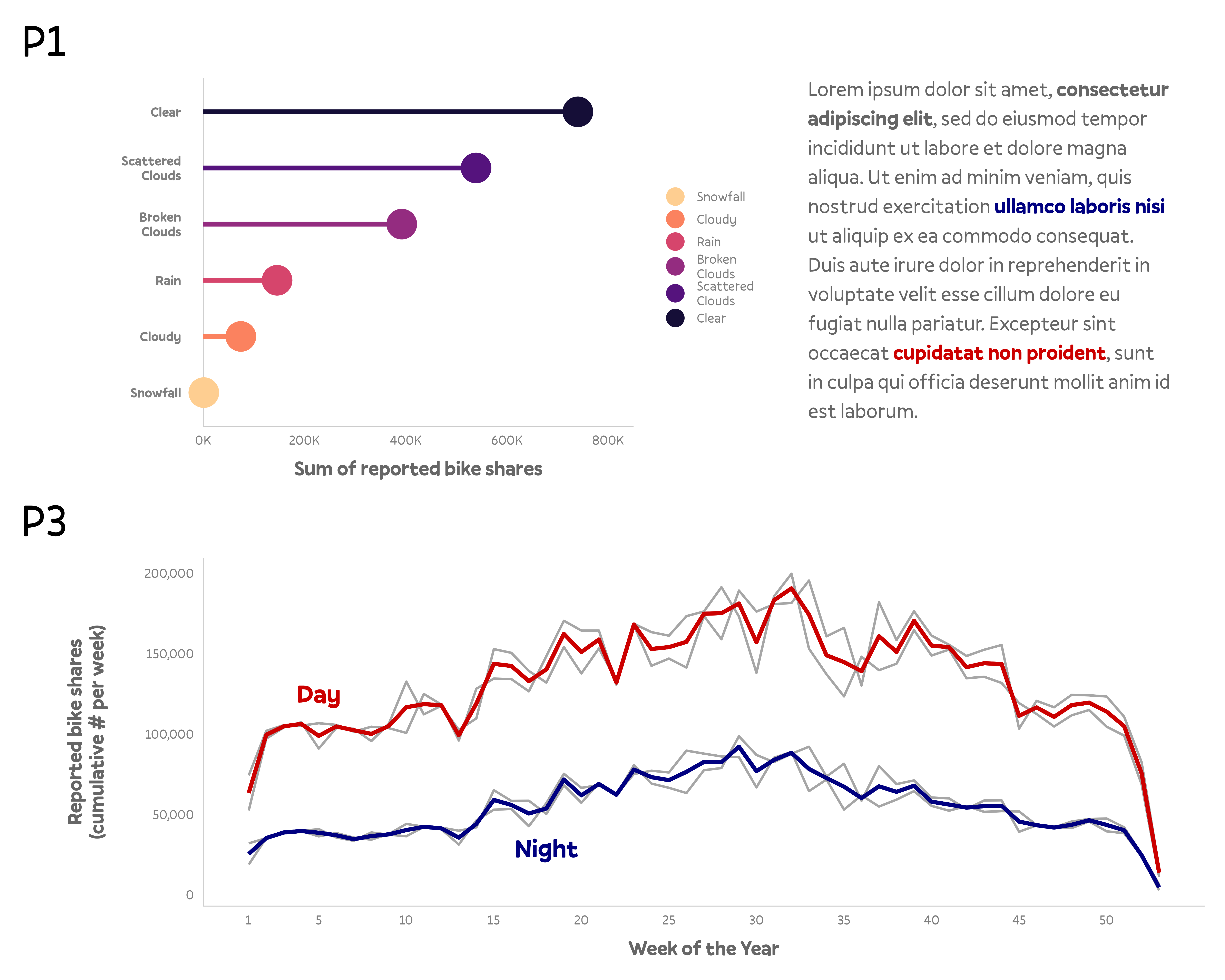
Add Inset Plots
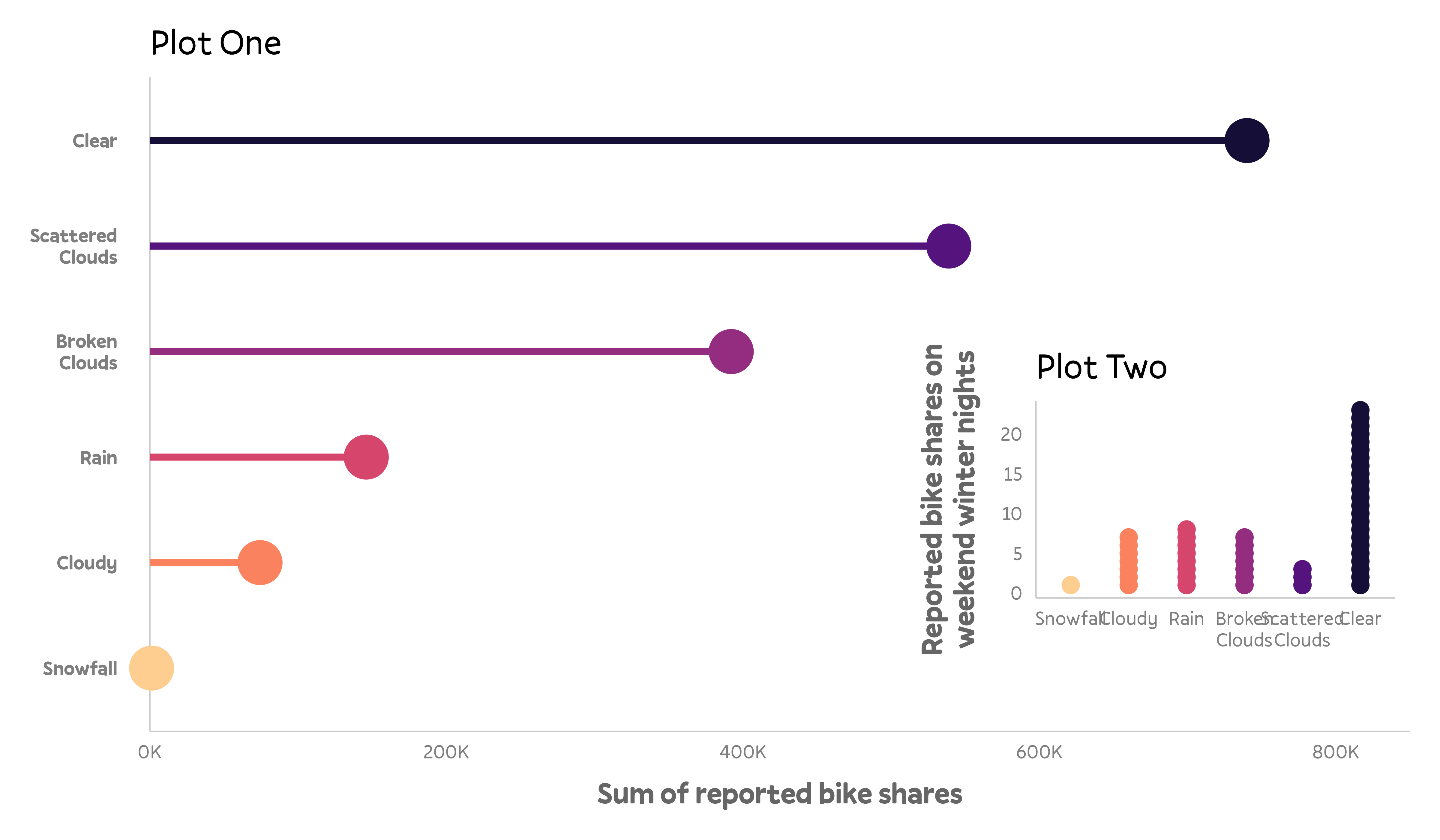
Add Inset Plots
Add Inset Plots
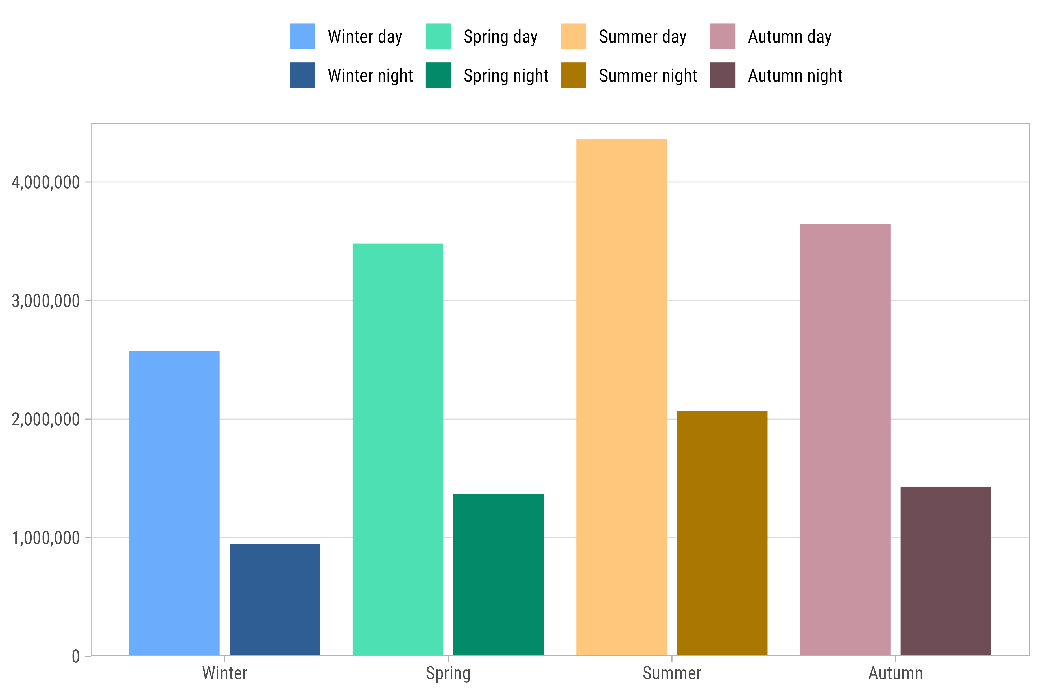
Legend with Color Shading
library(colorspace)
shades <- c(lighten(pal, .3),
                  darken(pal, .3))

g <-
  bikes %>%
  arrange(day_night, date) %>%
  mutate(
    season_day = paste(
      str_to_title(season), day_night
    ),
    season_day = forcats::fct_inorder(season_day)
  ) %>%
  ggplot(
    aes(x = season, y = count,
        fill = season_day)
  ) +
  stat_summary(
    geom = "col", fun = sum,
    position = position_dodge2(
      width = .2, padding = .1
    )
  ) +
  scale_fill_manual(
    values = shades, name = NULL
  ) +
  scale_x_discrete(
    labels = str_to_title
  ) +
  scale_y_continuous(
    labels = scales::comma_format(),
    expand = c(0, 0),
    limits = c(NA, 4500000)
  ) +
  labs(x = NULL, y = "Reported bike shares") +
  theme(
    panel.grid.major.x = element_blank(),
    axis.title = element_blank()
  )

g
Legend on Top

Resort Legend