Graphic Design with ggplot2

Concepts of the {ggplot2} Package Pt. 1:
Solution Exercise 1

Cédric Scherer // rstudio::conf // July 2022

Exercise 1

• Explore the TfL bike share data visually:
  create a timeseries of reported bike shares on weekend days
  • Highlight day and night encoded by colors and shapes.
  • Connect the points of each period with lines.
    • What is the difference between geom_line() and geom_path()?
  • Apply your favorite theme to the plot.
  • Add meaningful labels.
  • Bonus: use shape to encode Saturday vs Sunday instead.
• Save the plot as a vector graphic with a decent plot size.

Import the Data Set

bikes <- readr::read_csv(
  here::here("data", "london-bikes-custom.csv"),
  col_types = "Dcfffilllddddc"
)

bikes$season <- forcats::fct_inorder(bikes$season)

library(tidyverse)

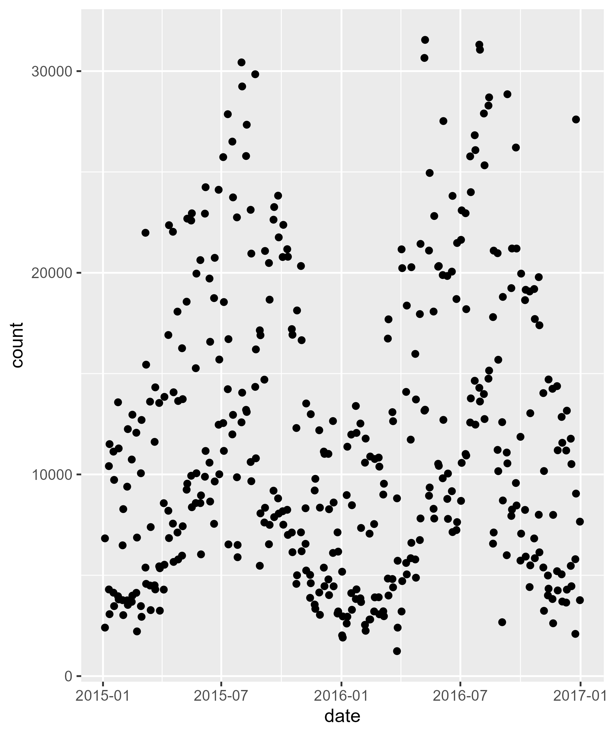
Scatterplot Counts vs. Date

ggplot(
    filter(bikes, is_weekend == TRUE),
    aes(x = date, y = count)
  ) +
  geom_point()

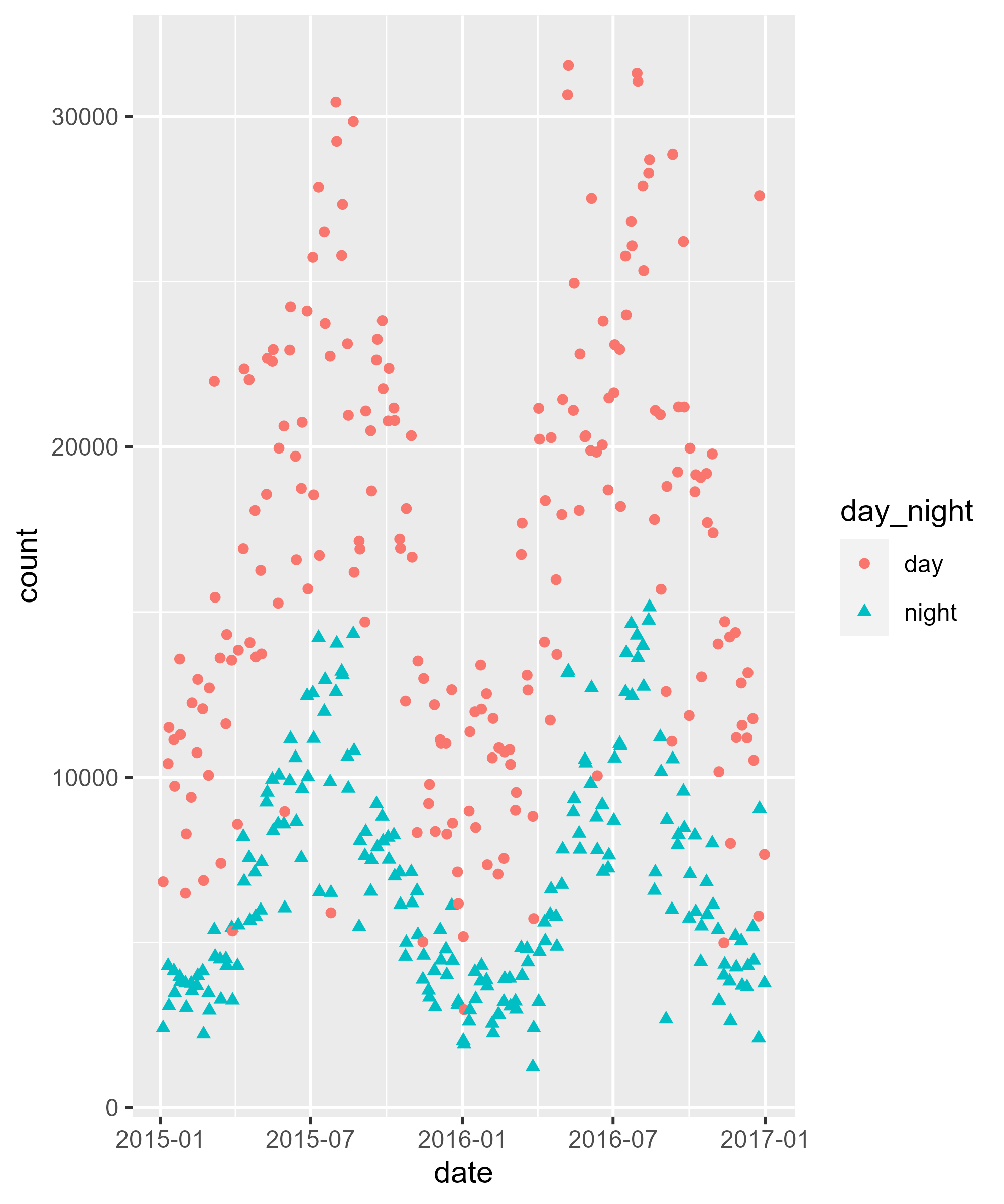
Encode Day Period by Colors and Shapes

ggplot(
    filter(bikes, is_weekend == TRUE),
    aes(x = date, y = count)
  ) +
  geom_point(
    aes(color = day_night,
        shape = day_night)
  )

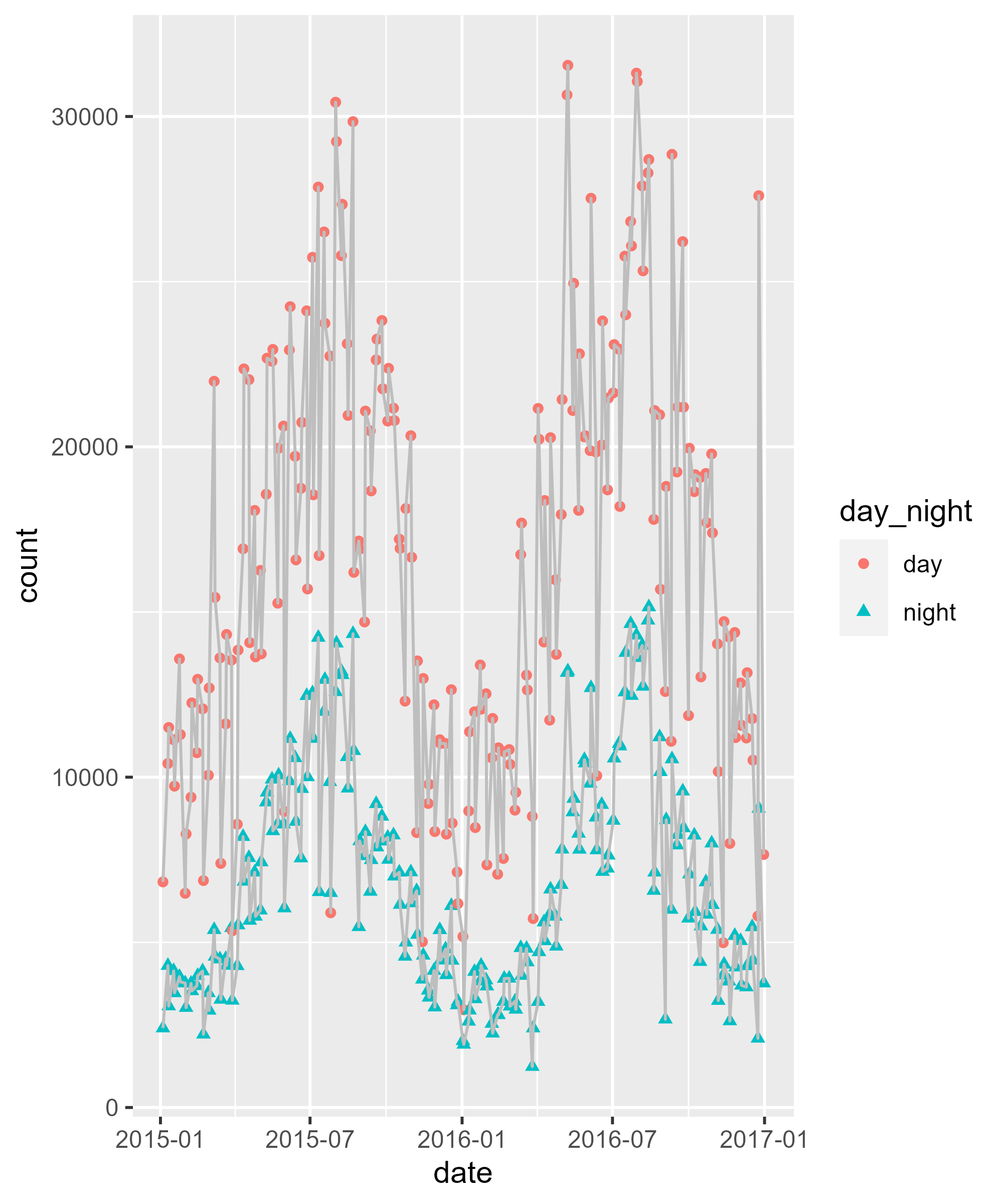
Add Line

ggplot(
    filter(bikes, is_weekend == TRUE),
    aes(x = date, y = count)
  ) +
  geom_point(
    aes(color = day_night,
        shape = day_night)
  ) +
  geom_line(
    color = "grey"
  )

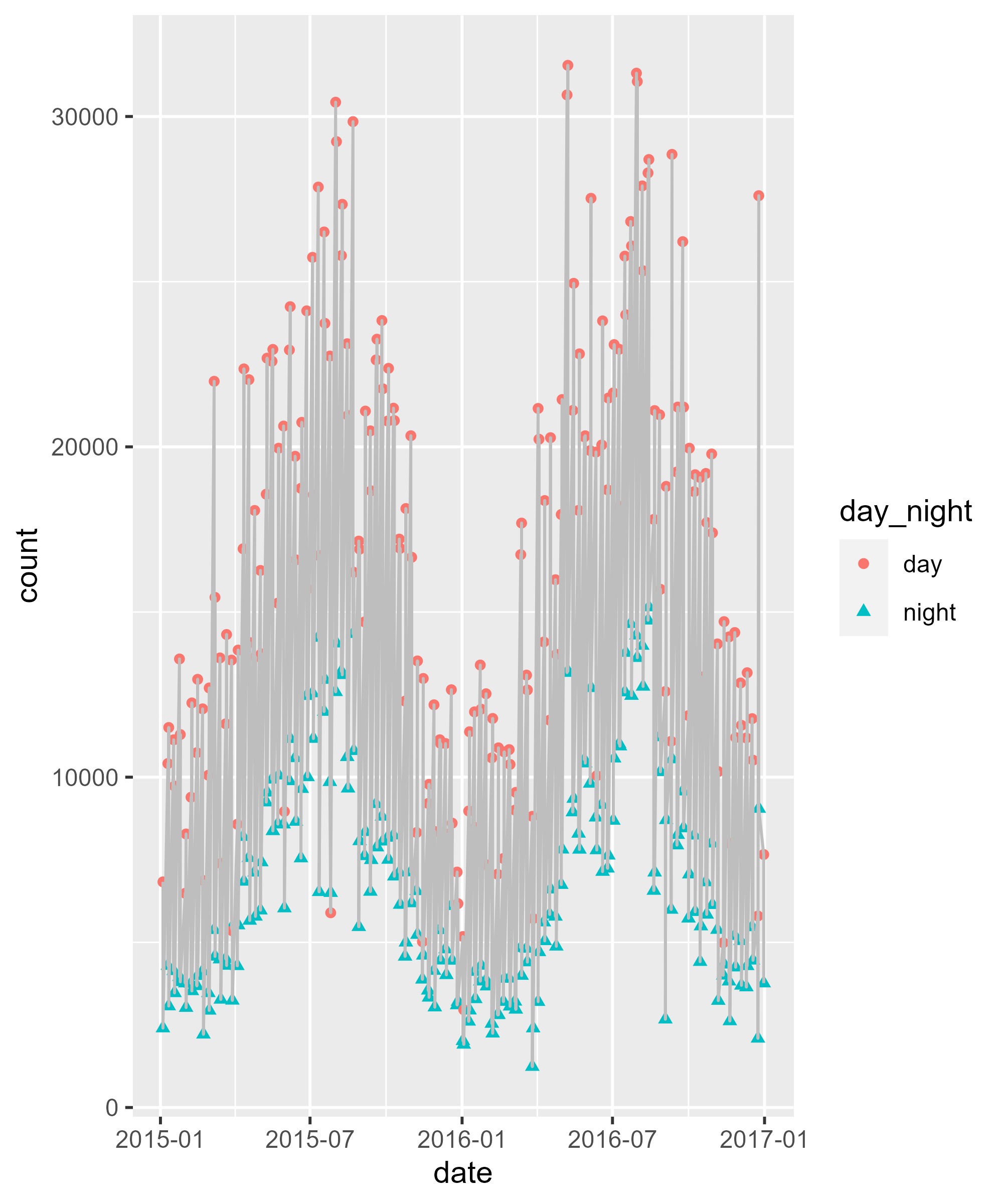
Group Lines by Day Period

ggplot(
    filter(bikes, is_weekend == TRUE),
    aes(x = date, y = count)
  ) +
  geom_point(
    aes(color = day_night,
        shape = day_night)
  ) +
  geom_line(
    aes(group = day_night),
    color = "grey"
  )

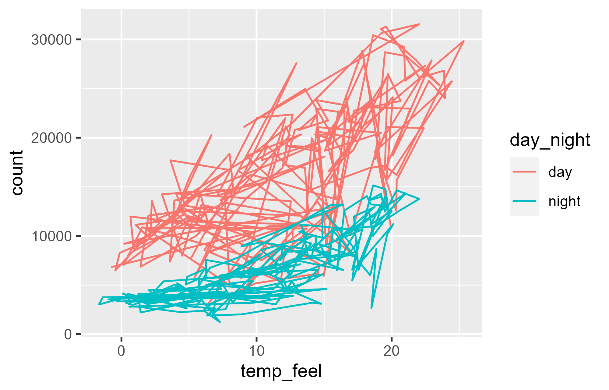
Order Layers

ggplot(
    filter(bikes, is_weekend == TRUE),
    aes(x = date, y = count)
  ) +
  geom_line(
    aes(group = day_night),
    color = "grey"
  ) +
  geom_point(
    aes(color = day_night,
        shape = day_night)
  )

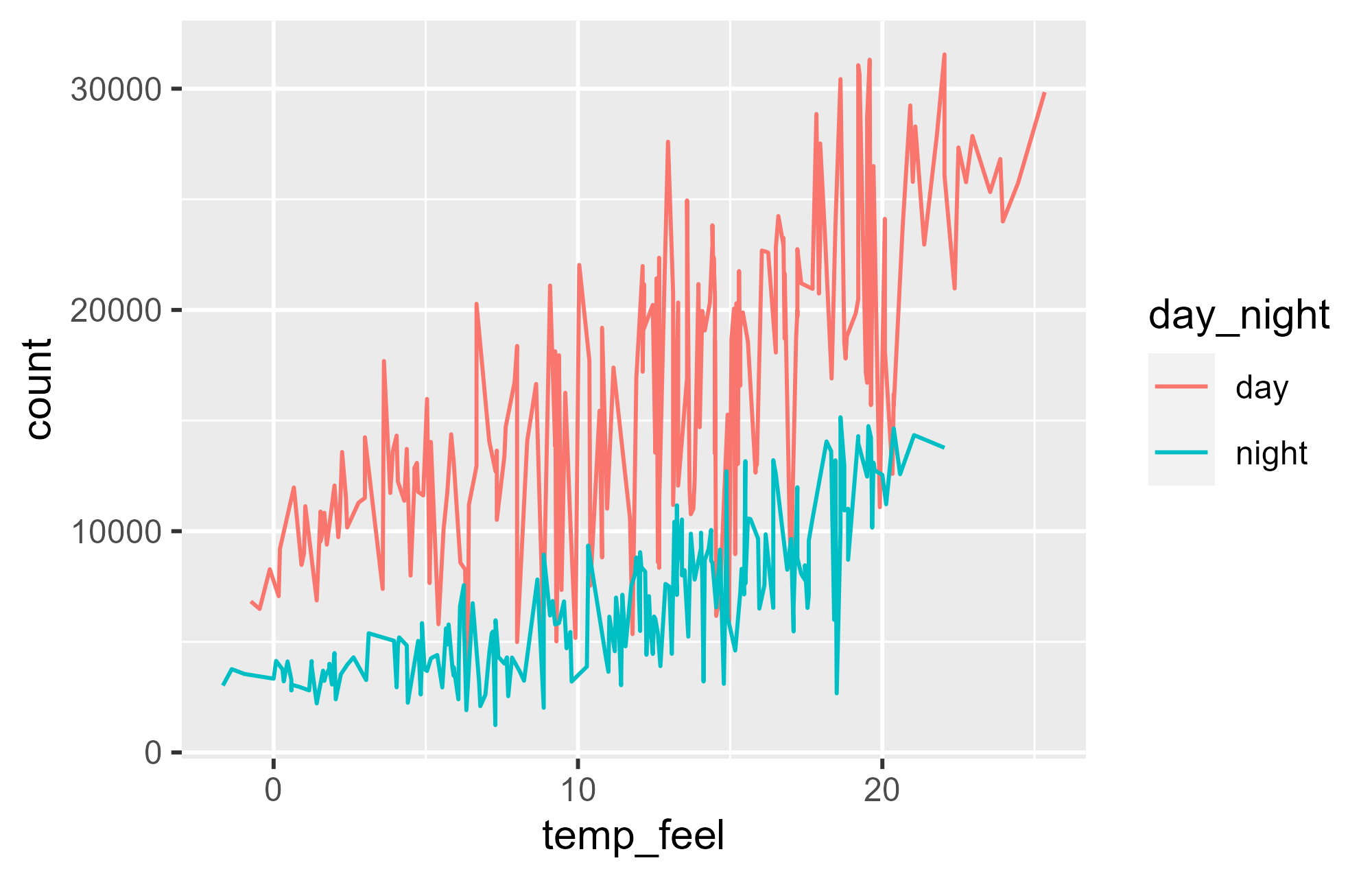
Use `geom_path()` instead

ggplot(
    filter(bikes, is_weekend == TRUE),
    aes(x = date, y = count)
  ) +
  geom_path(
    aes(group = day_night),
    color = "grey"
  ) +
  geom_point(
    aes(color = day_night,
        shape = day_night)
  )

`geom_line()` vs. `geom_path()`

ggplot(
    filter(bikes, is_weekend == TRUE),
    aes(x = temp_feel, y = count)
  ) +
  geom_path(
    aes(color = day_night)
  )

ggplot(
    filter(bikes, is_weekend == TRUE),
    aes(x = temp_feel, y = count)
  ) +
  geom_line(
    aes(color = day_night)
  )

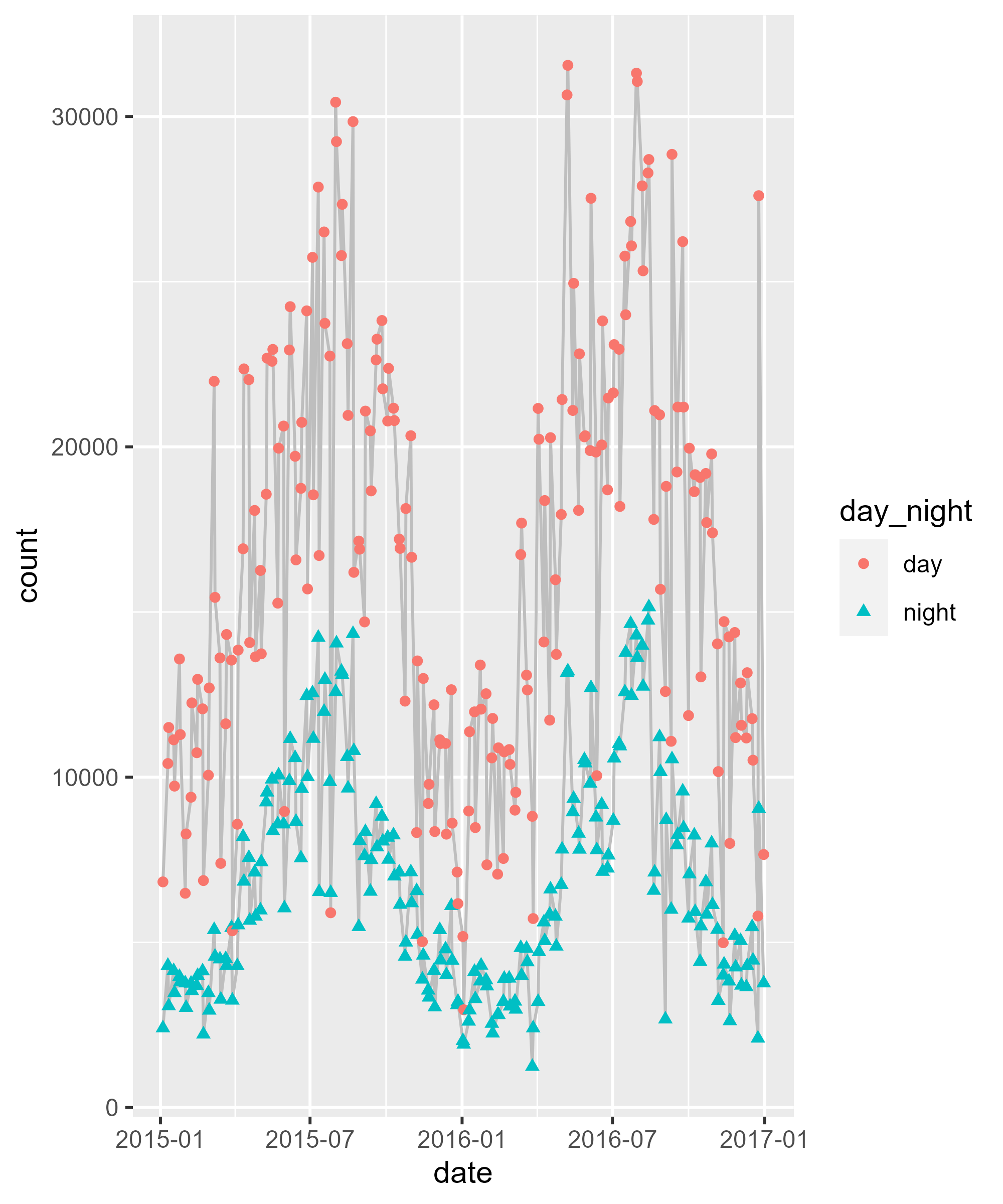
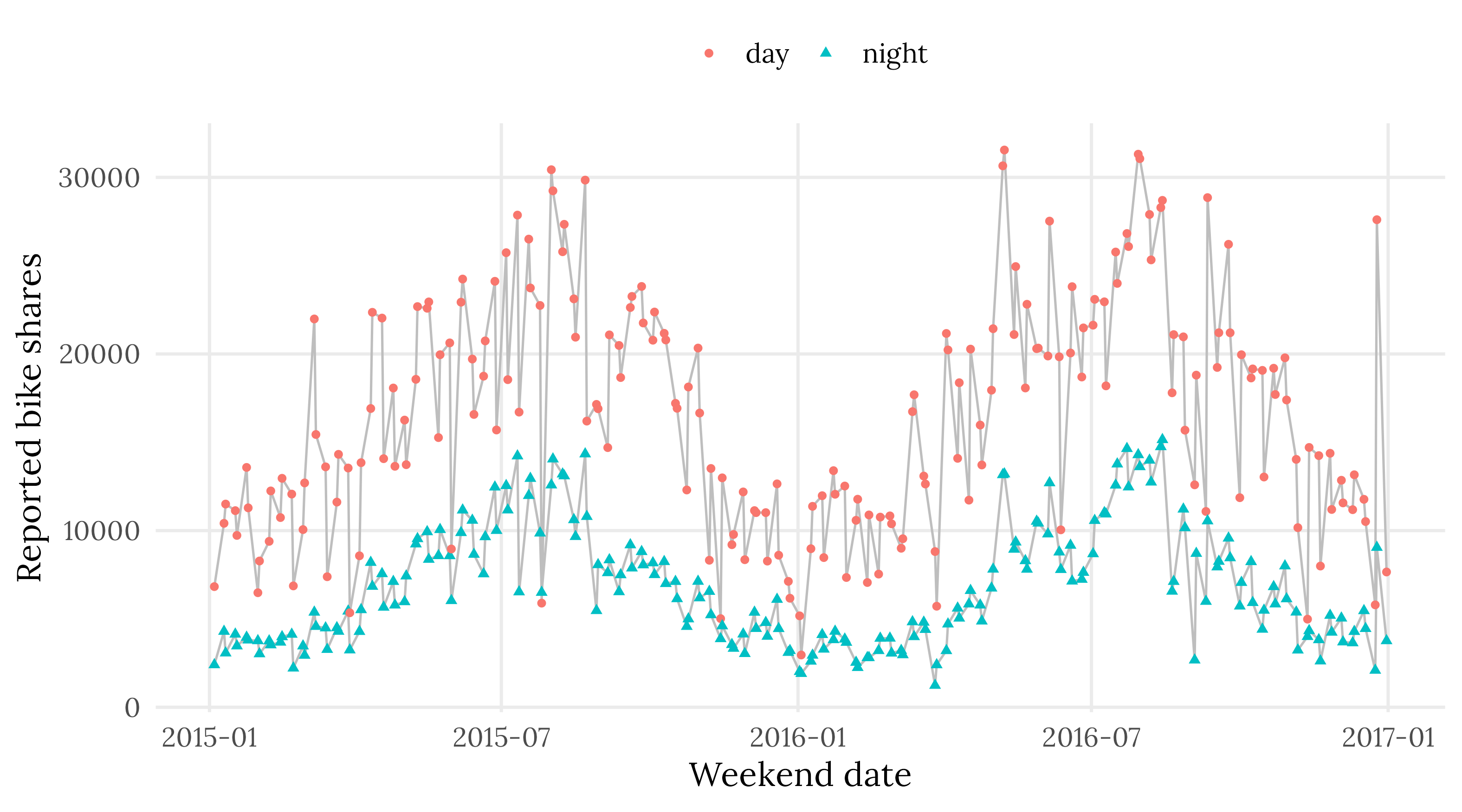
Apply a Theme

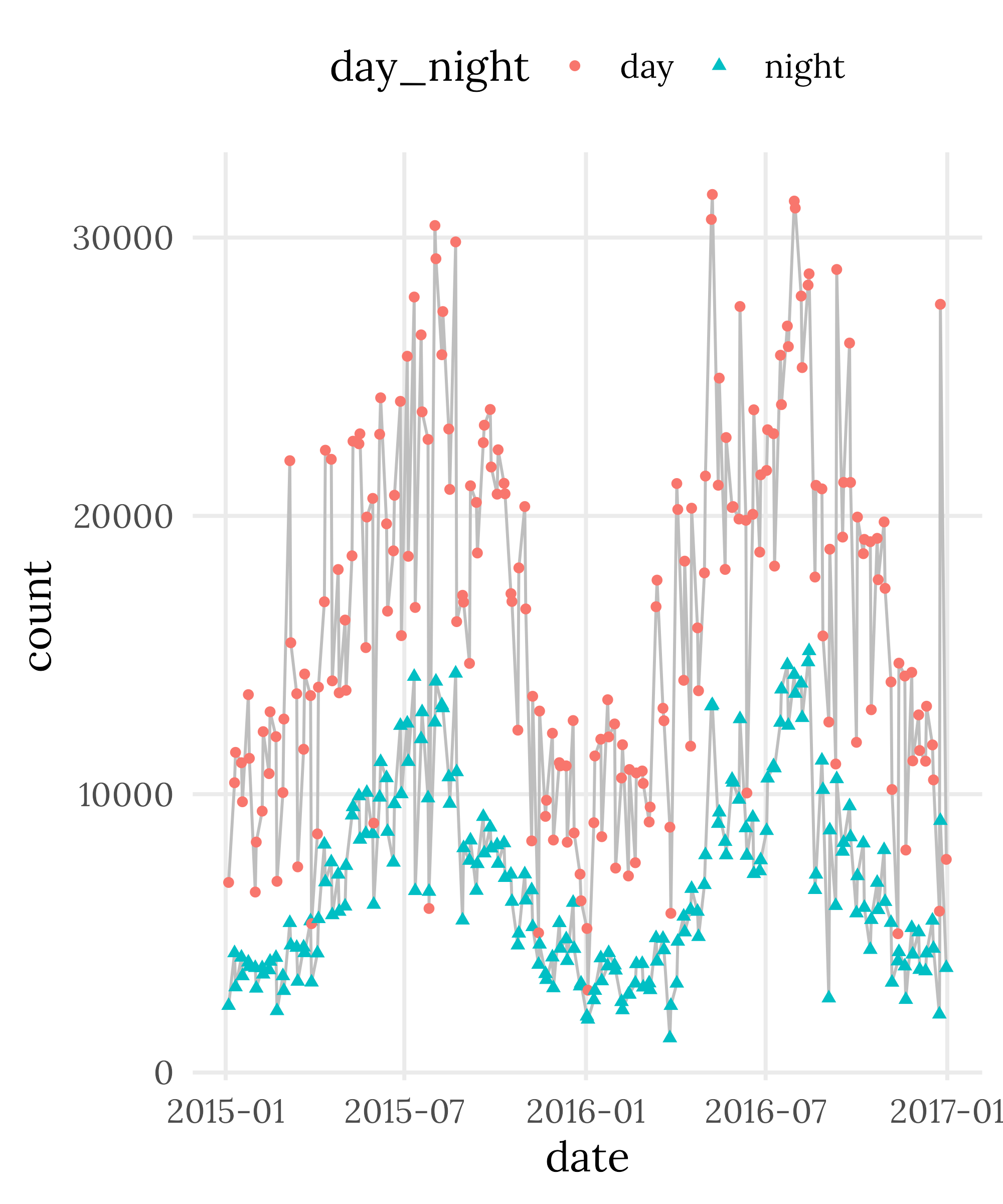
g <- ggplot(
    filter(bikes, is_weekend == TRUE),
    aes(x = date, y = count)
  ) +
  geom_line(
    aes(group = day_night),
    color = "grey"
  ) +
  geom_point(
    aes(color = day_night,
        shape = day_night)
  )

g +
  theme_minimal(
    base_size = 15,
    base_family = "Lora"
  ) +
  theme(
    legend.position = "top",
    panel.grid.minor = element_blank()
  )

Add Meaningful Labels

g +
  labs(
    x = "Weekend date",
    y = "Reported bike shares",
    color = "Part of the Day:"
  ) +
  theme_minimal(
    base_size = 15,
    base_family = "Lora"
  ) +
  theme(
    legend.position = "top",
    panel.grid.minor = element_blank()
  )

Add Meaningful Labels

g +
  labs(
    x = "Weekend date",
    y = "Reported bike shares",
    color = "Part of the Day:",
    shape = "Part of the Day:"
  ) +
  theme_minimal(
    base_size = 15,
    base_family = "Lora"
  ) +
  theme(
    legend.position = "top",
    panel.grid.minor = element_blank()
  )

Add Meaningful Labels

g +
  labs(
    x = "Weekend date",
    y = "Reported bike shares",
    color = NULL,
    shape = NULL
  ) +
  theme_minimal(
    base_size = 15,
    base_family = "Lora"
  ) +
  theme(
    legend.position = "top",
    panel.grid.minor = element_blank()
  )

Save the Plot

ggsave(here::here("exercises", "plots", "02_concepts_pt1_ex1.pdf"),
       width = 9, height = 5, device = cairo_pdf)

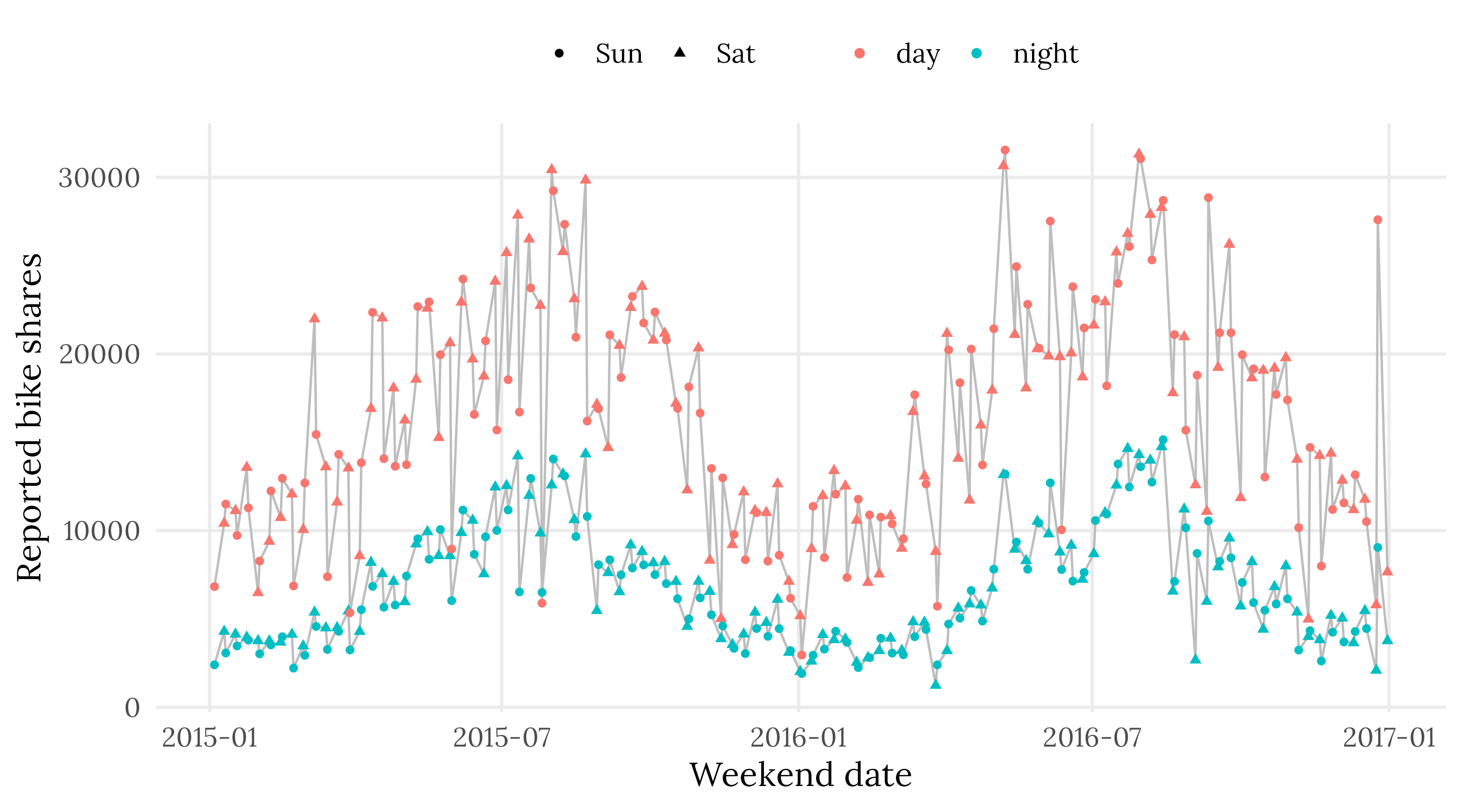
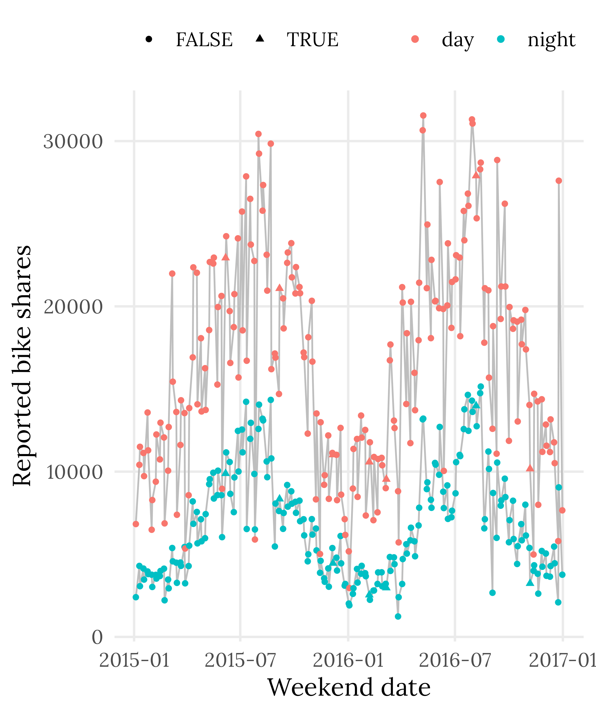
Bonus: Use Shape to Encode Sat vs Sun

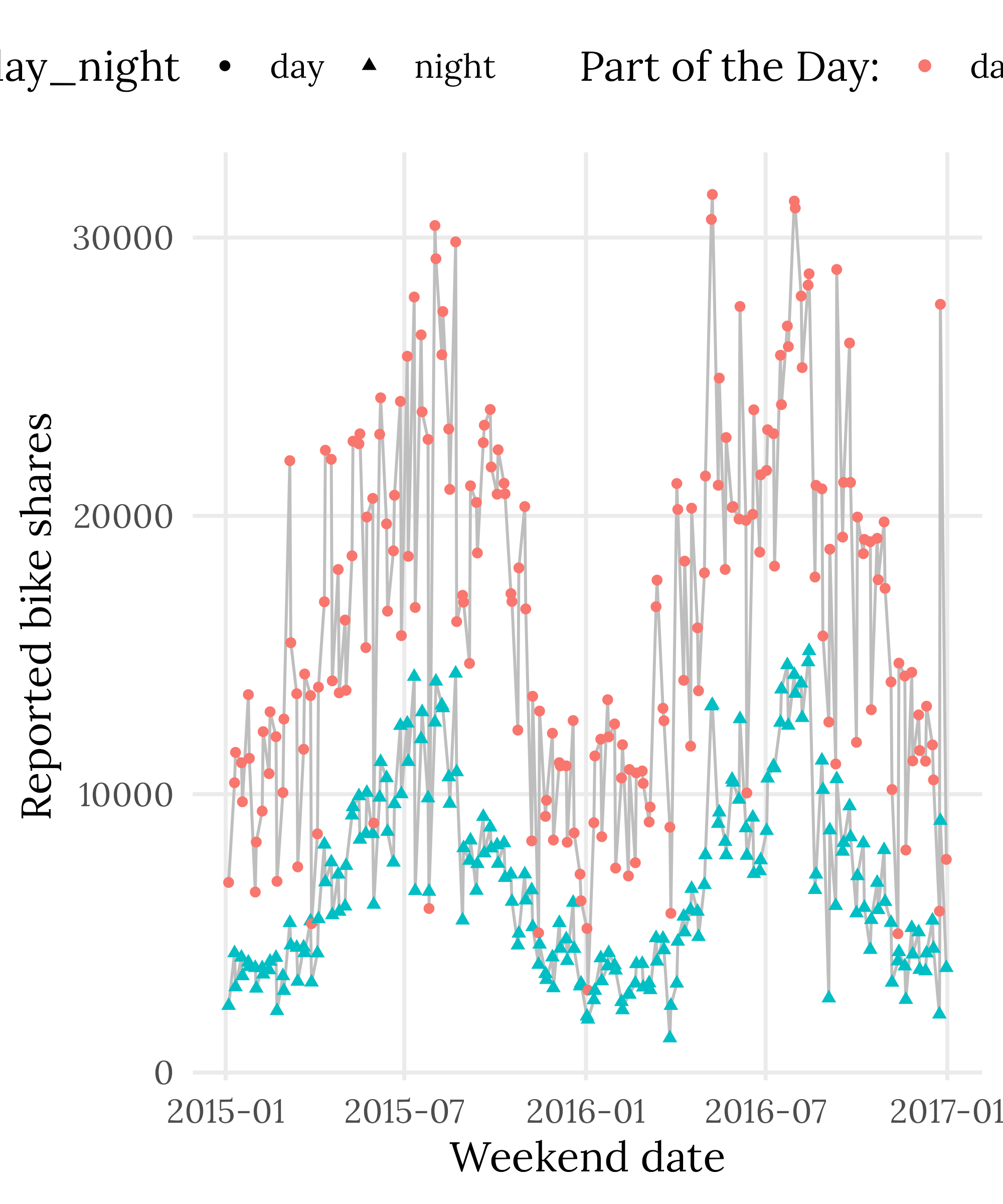
ggplot(
    filter(bikes, is_weekend == TRUE),
    aes(x = date, y = count)
  ) +
  geom_line(
    aes(group = day_night),
    color = "grey"
  ) +
  geom_point(
    aes(color = day_night,
        shape = lubridate::day(date) == 6)
  ) +
  labs(
    x = "Weekend date",
    y = "Reported bike shares",
    color = NULL,
    shape = NULL
  ) +
  theme_minimal(
    base_size = 15,
    base_family = "Lora"
  ) +
  theme(
    legend.position = "top",
    panel.grid.minor = element_blank()
  )

Bonus: Use Shape to Encode Sat vs Sun

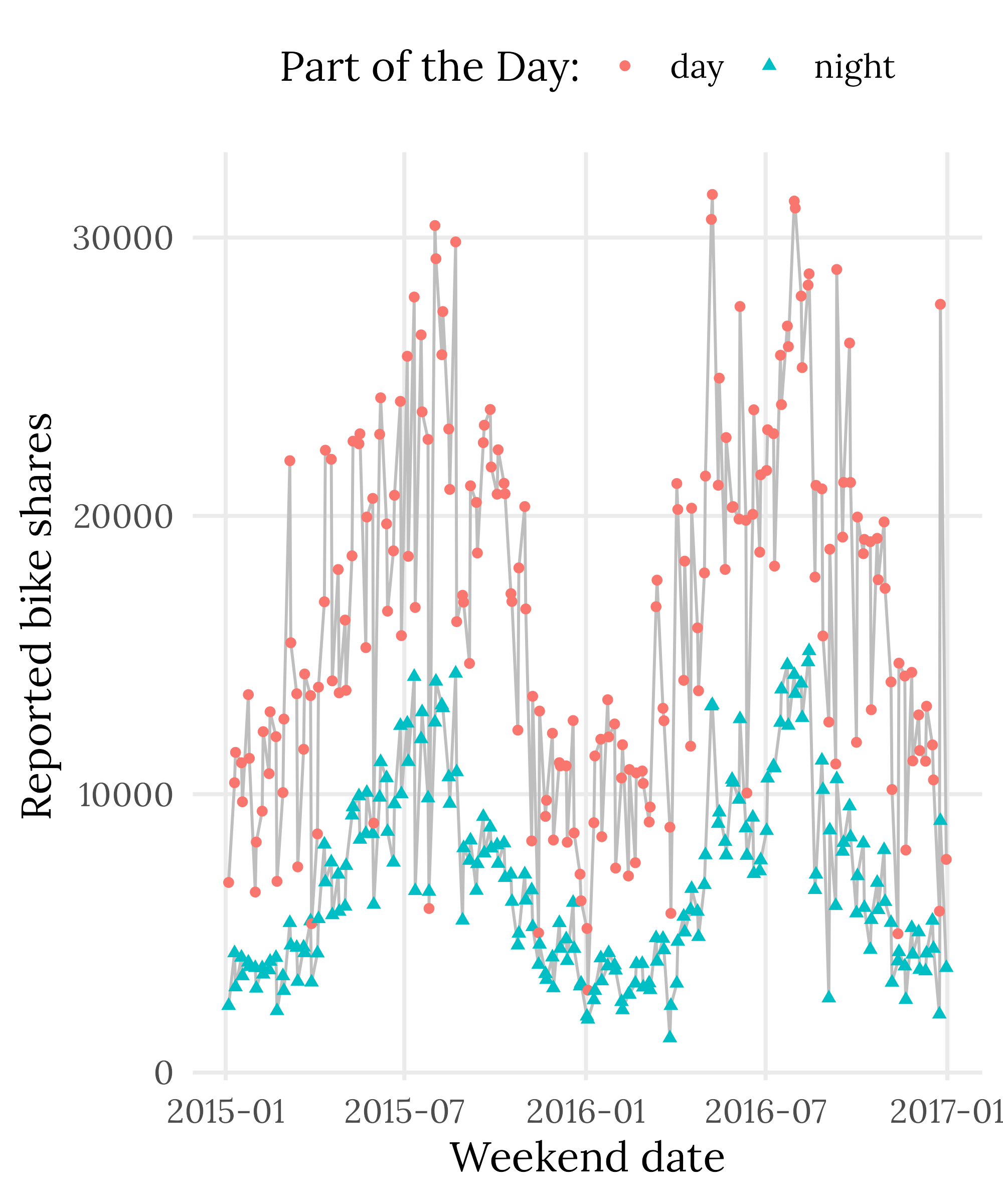
ggplot(
    filter(bikes, is_weekend == TRUE),
    aes(x = date, y = count)
  ) +
  geom_line(
    aes(group = day_night),
    color = "grey"
  ) +
  geom_point(
    aes(color = day_night,
        shape = lubridate::wday(date, label = TRUE))
  ) +
  labs(
    x = "Weekend date",
    y = "Reported bike shares",
    color = NULL,
    shape = NULL
  ) +
  theme_minimal(
    base_size = 15,
    base_family = "Lora"
  ) +
  theme(
    legend.position = "top",
    panel.grid.minor = element_blank()
  )

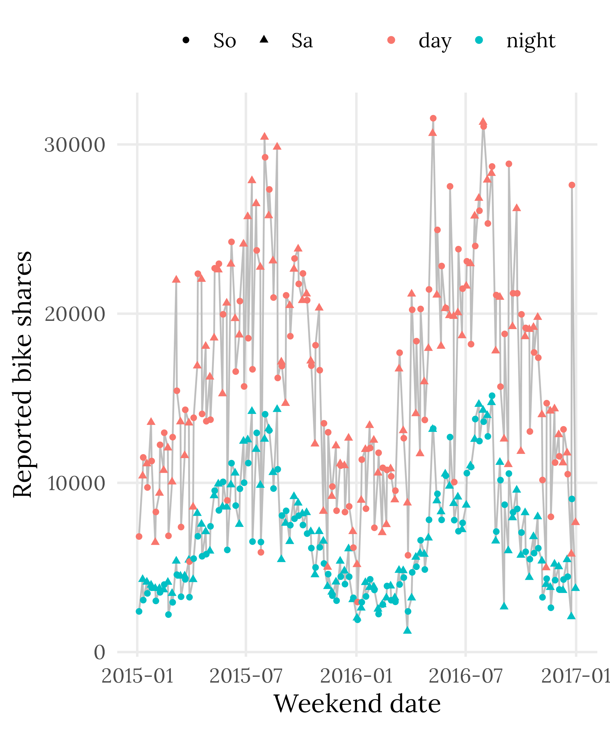
Bonus: Use Shape to Encode Sat vs Sun

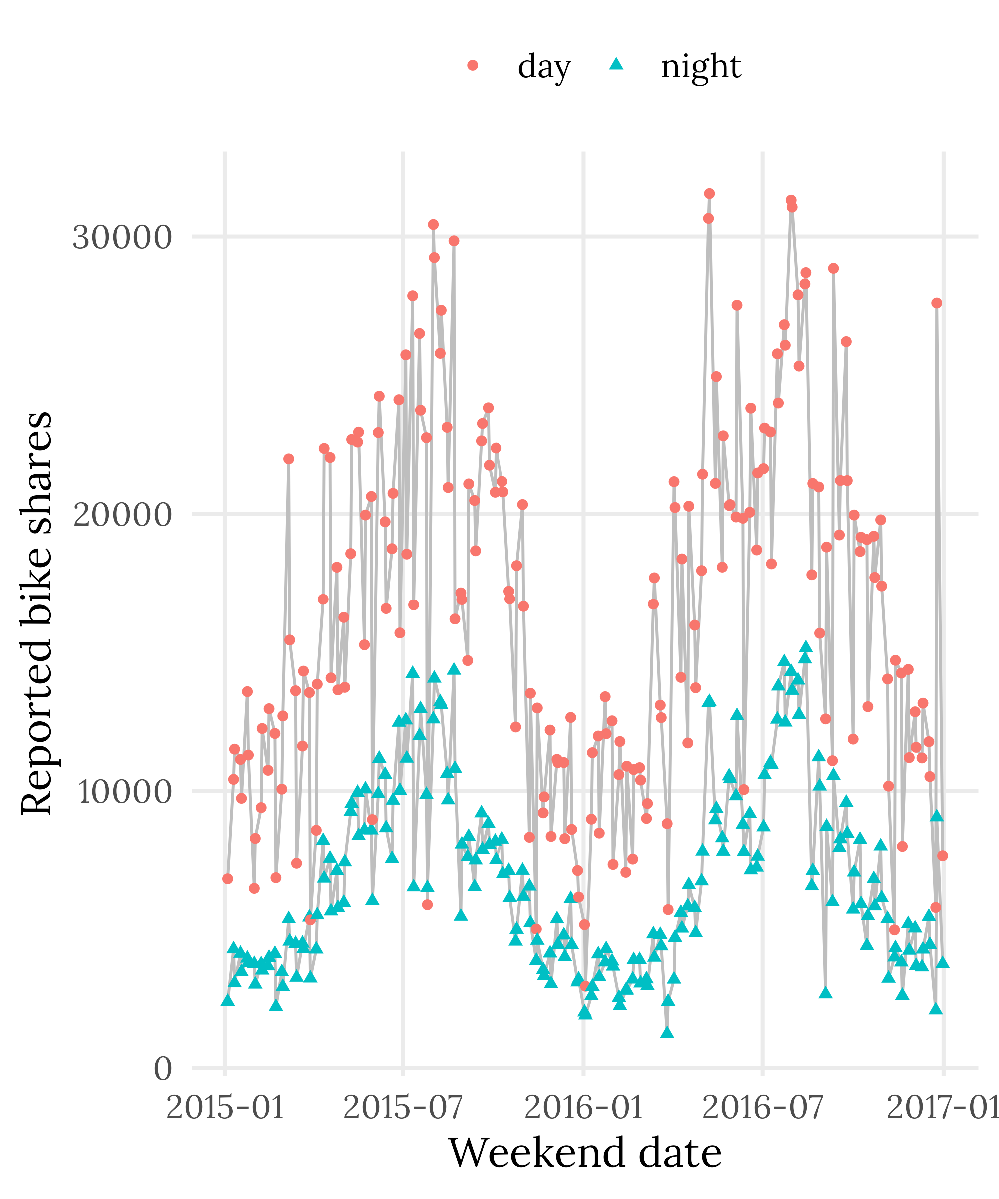
invisible(
  Sys.setlocale("LC_TIME", "C")
)

ggplot(
    filter(bikes, is_weekend == TRUE),
    aes(x = date, y = count)
  ) +
  geom_line(
    aes(group = day_night),
    color = "grey"
  ) +
  geom_point(
    aes(color = day_night,
        shape = lubridate::wday(date, label = TRUE))
  ) +
  labs(
    x = "Weekend date",
    y = "Reported bike shares",
    color = NULL,
    shape = NULL
  ) +
  theme_minimal(
    base_size = 15,
    base_family = "Lora"
  ) +
  theme(
    legend.position = "top",
    panel.grid.minor = element_blank()
  )

Save the Plot

ggsave(here::here("exercises", "plots", "02_concepts_pt1_ex1_bonus.pdf"),
       width = 9, height = 5, device = cairo_pdf)