Graphic Design with ggplot2
Concepts of the {ggplot2} Package Pt. 1:
Solution Exercise 2
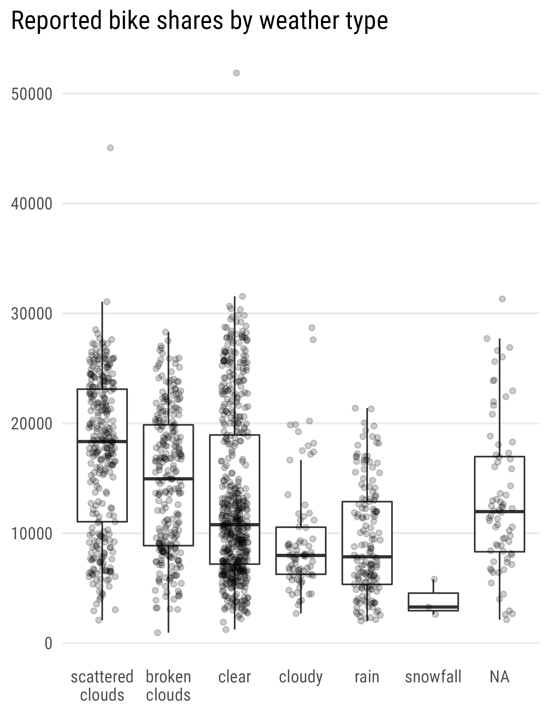
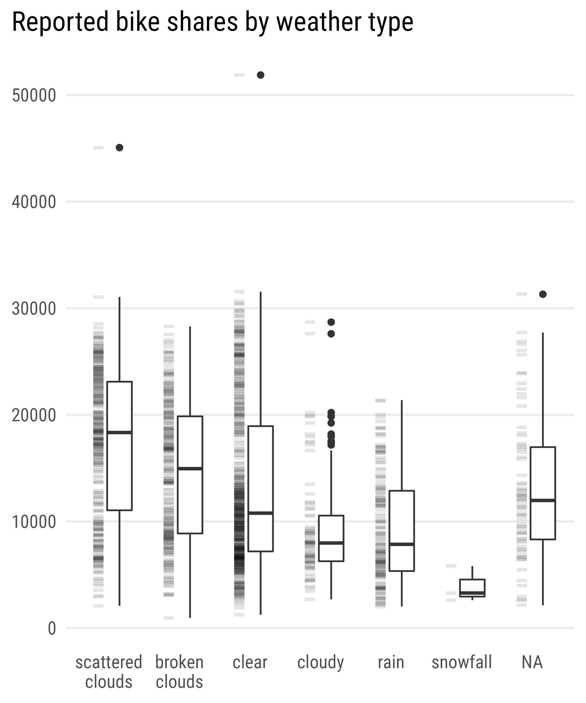
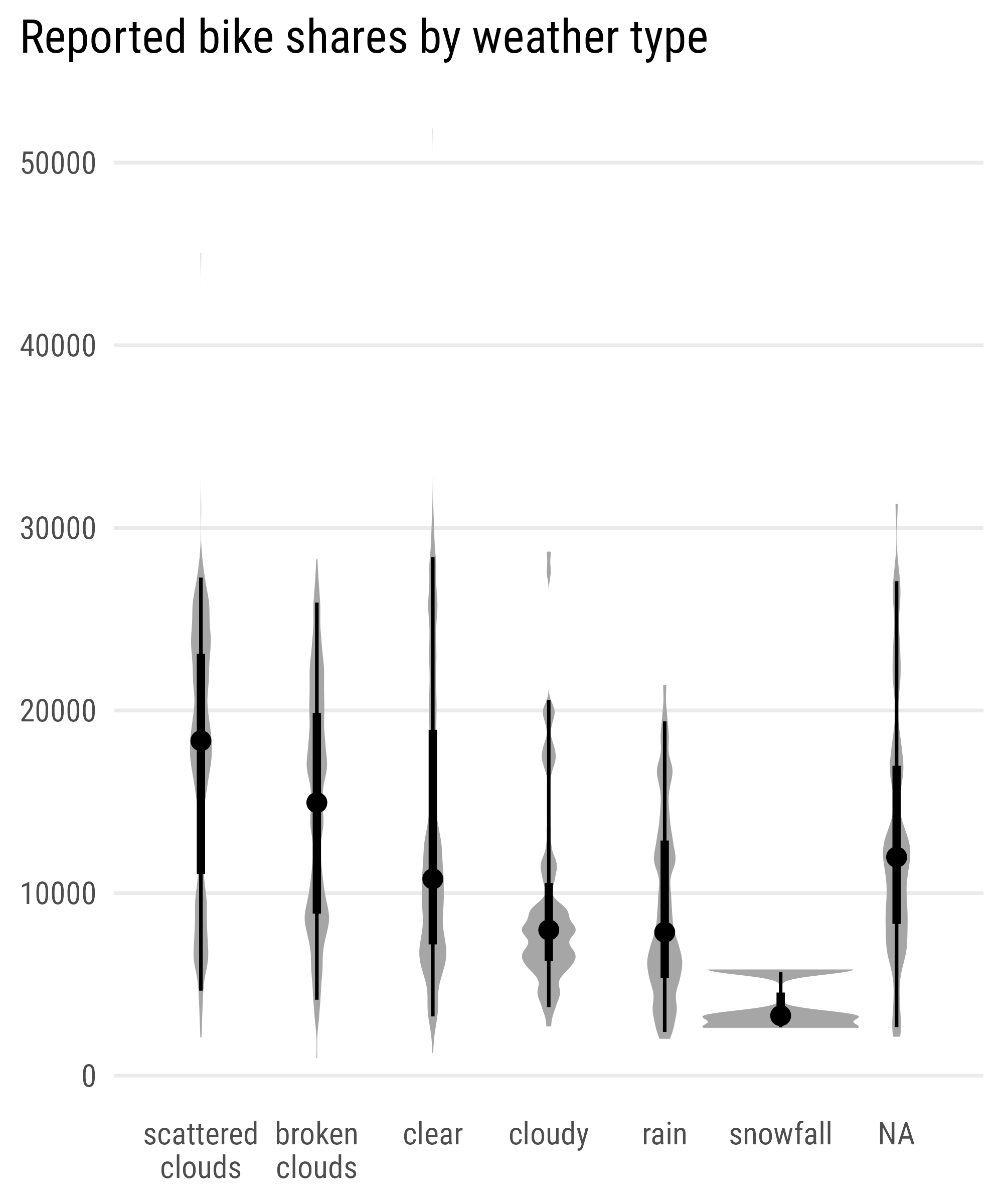
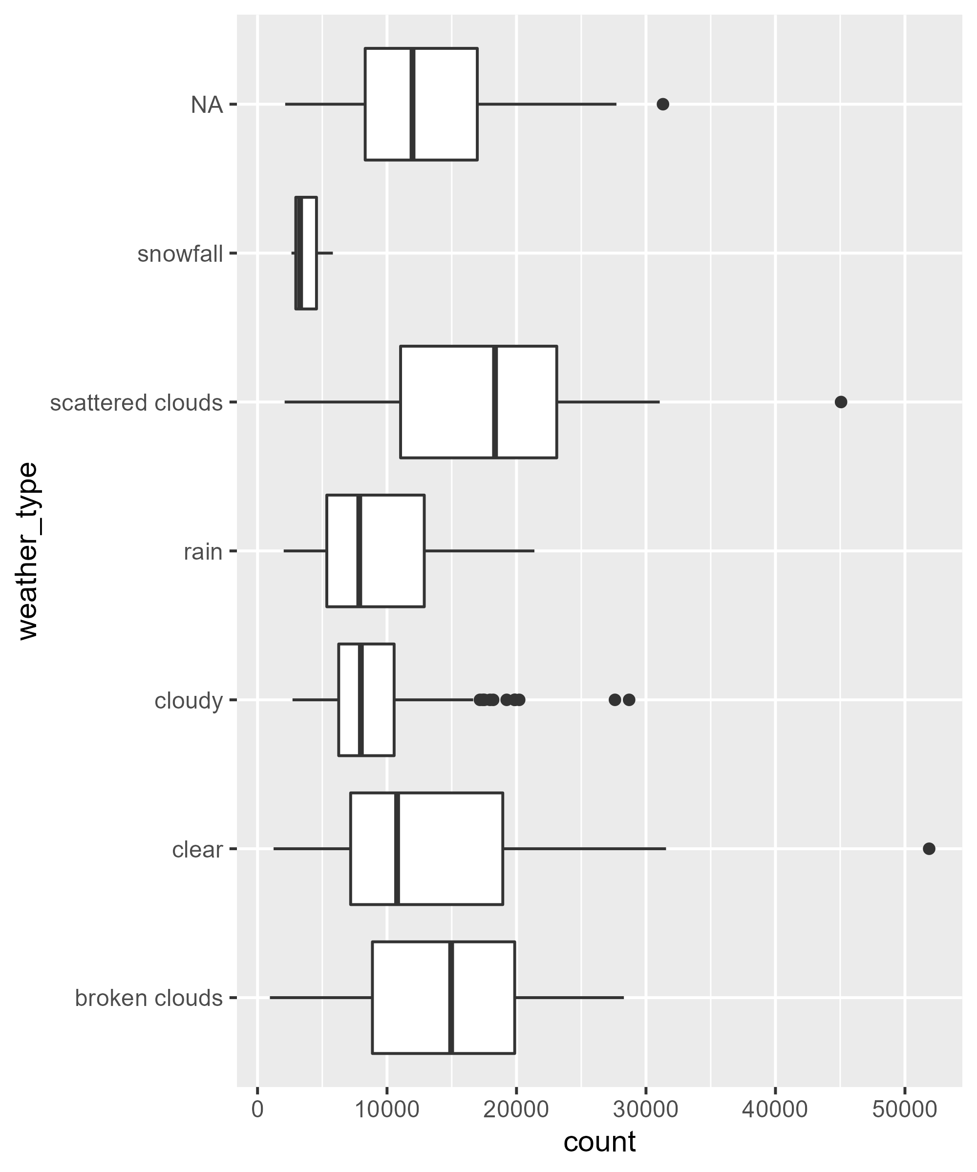
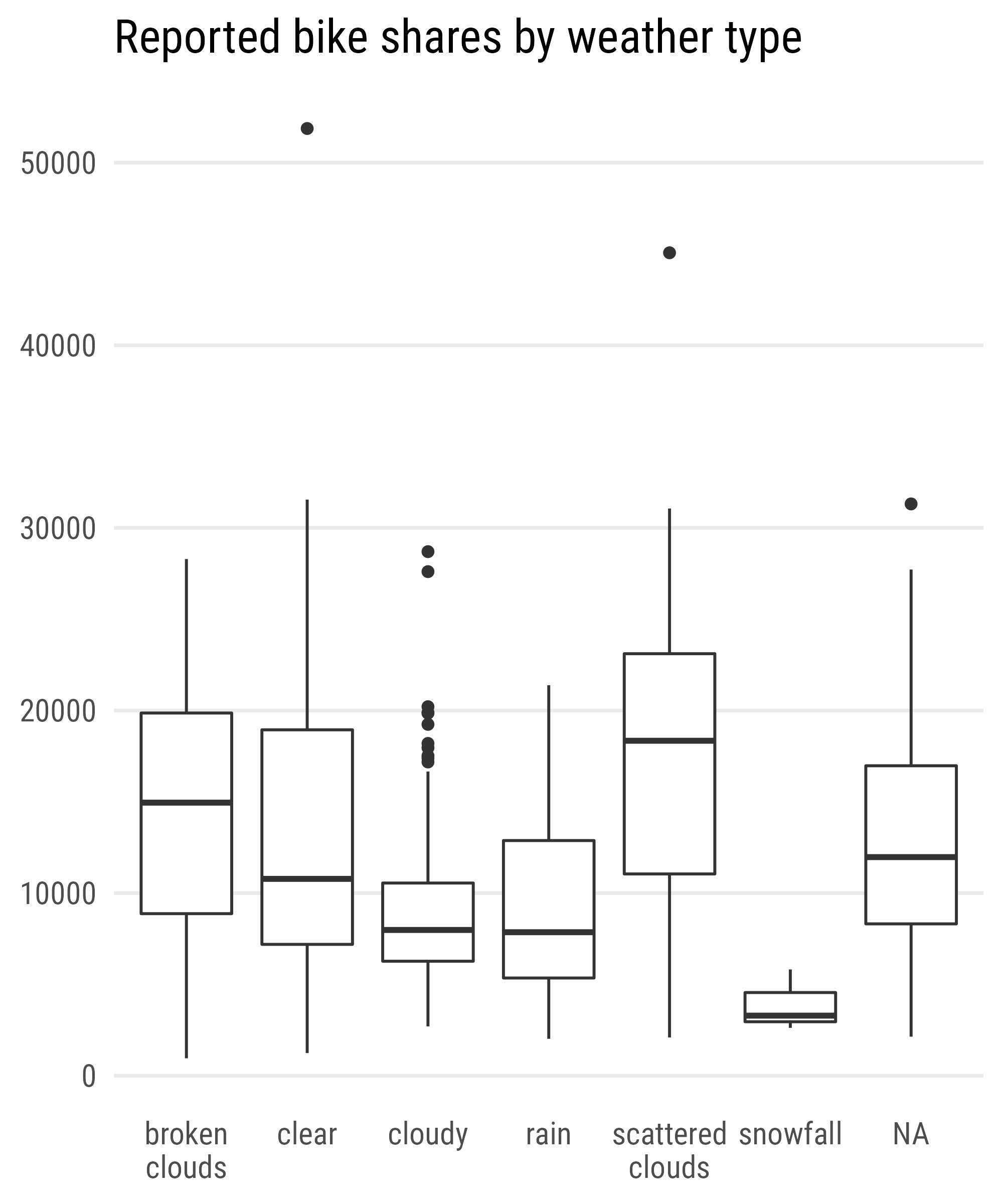
Boxplot of Counts vs. Weather Type
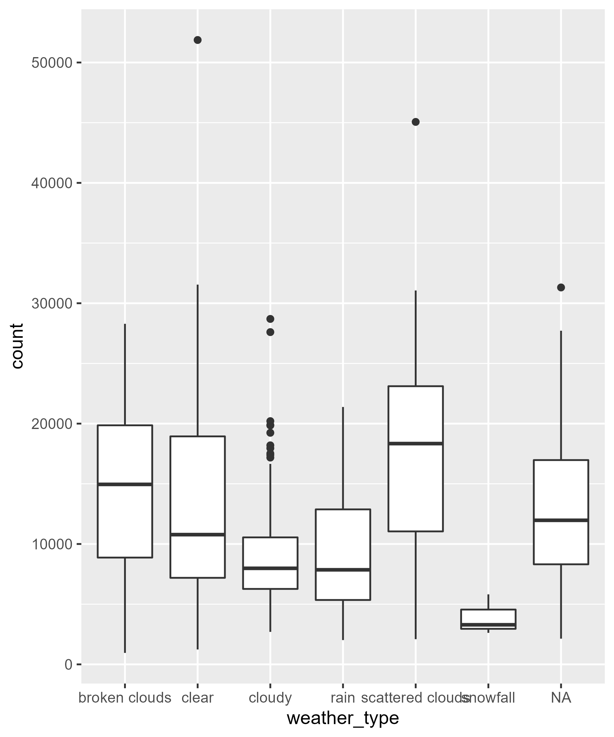
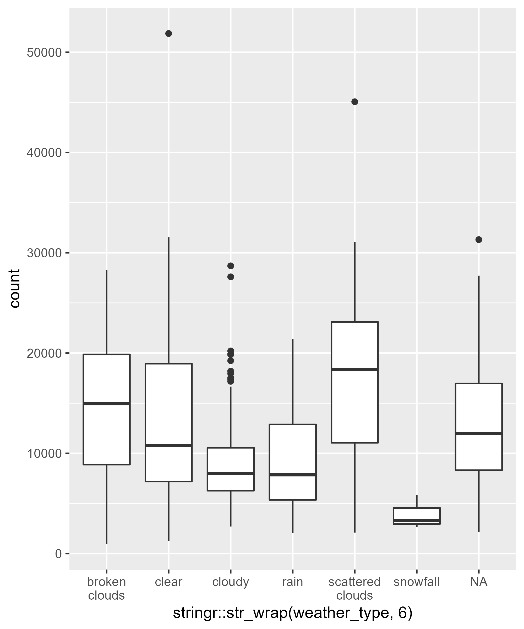
Avoid Overlapping Axis Labels
Avoid Overlapping Axis Labels
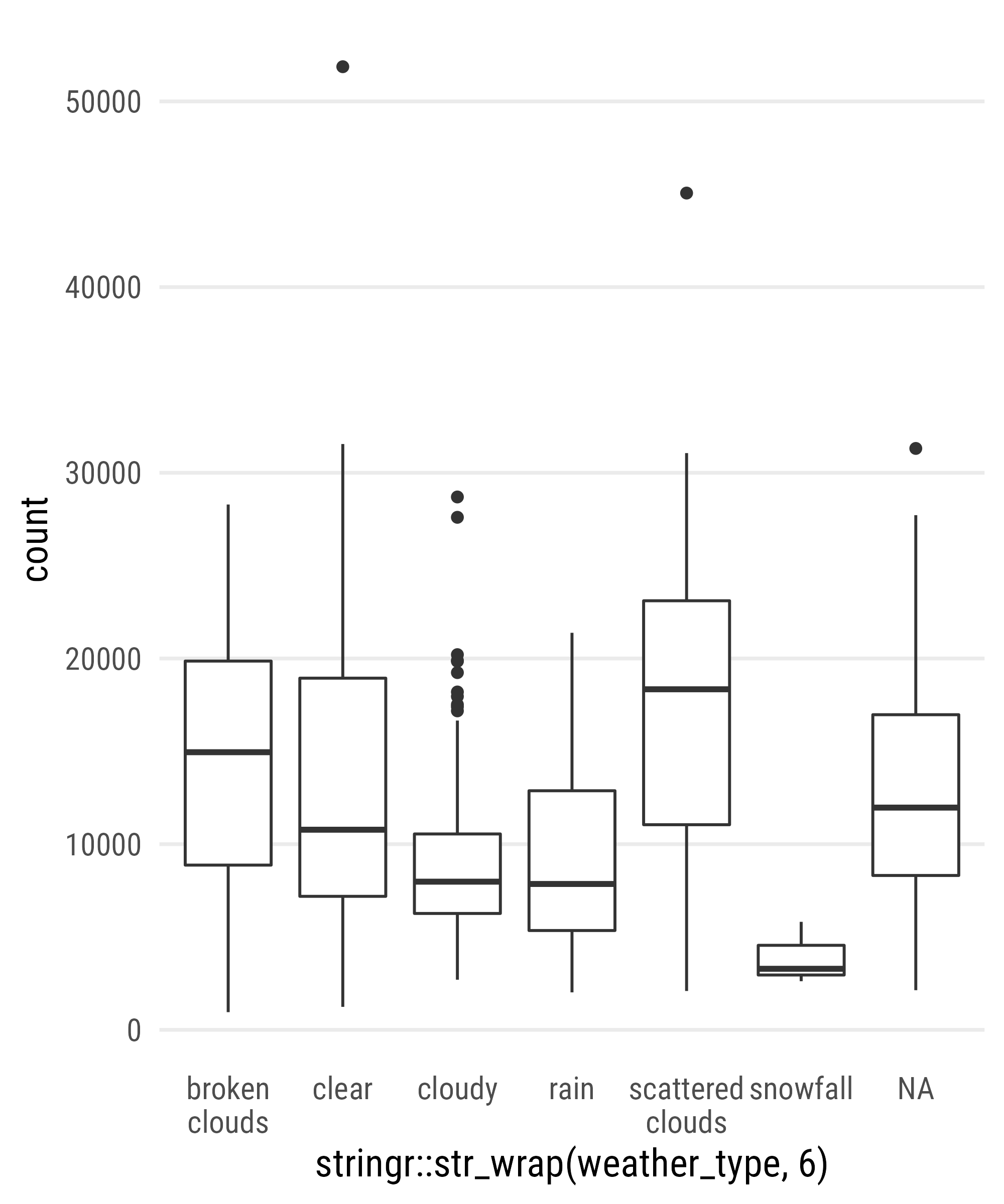
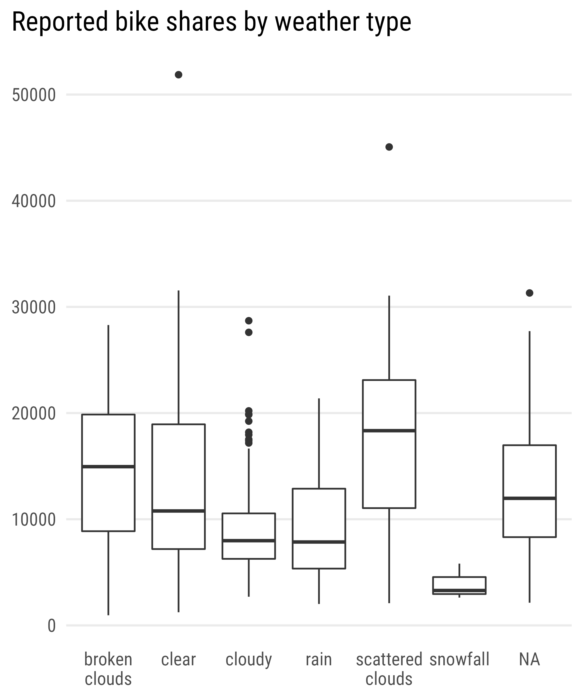
Apply a Theme

Customize the Theme
Add Meaningful Labels
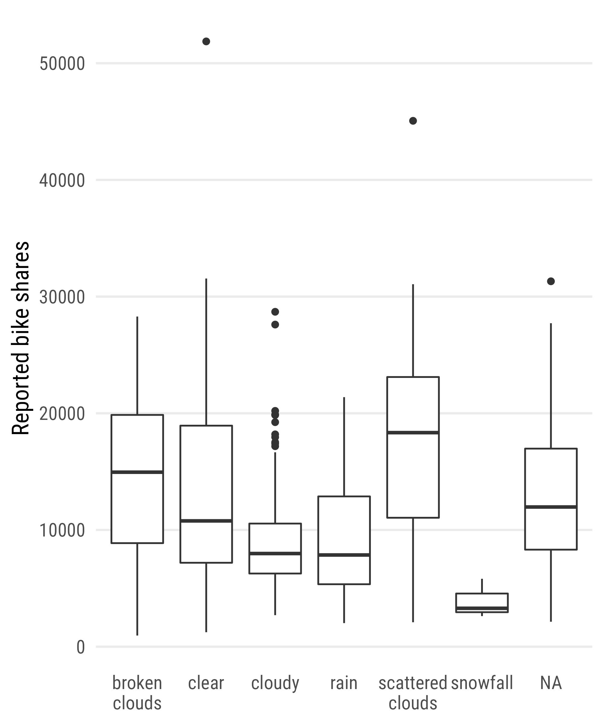
Add Meaningful Labels
Add Meaningful Labels
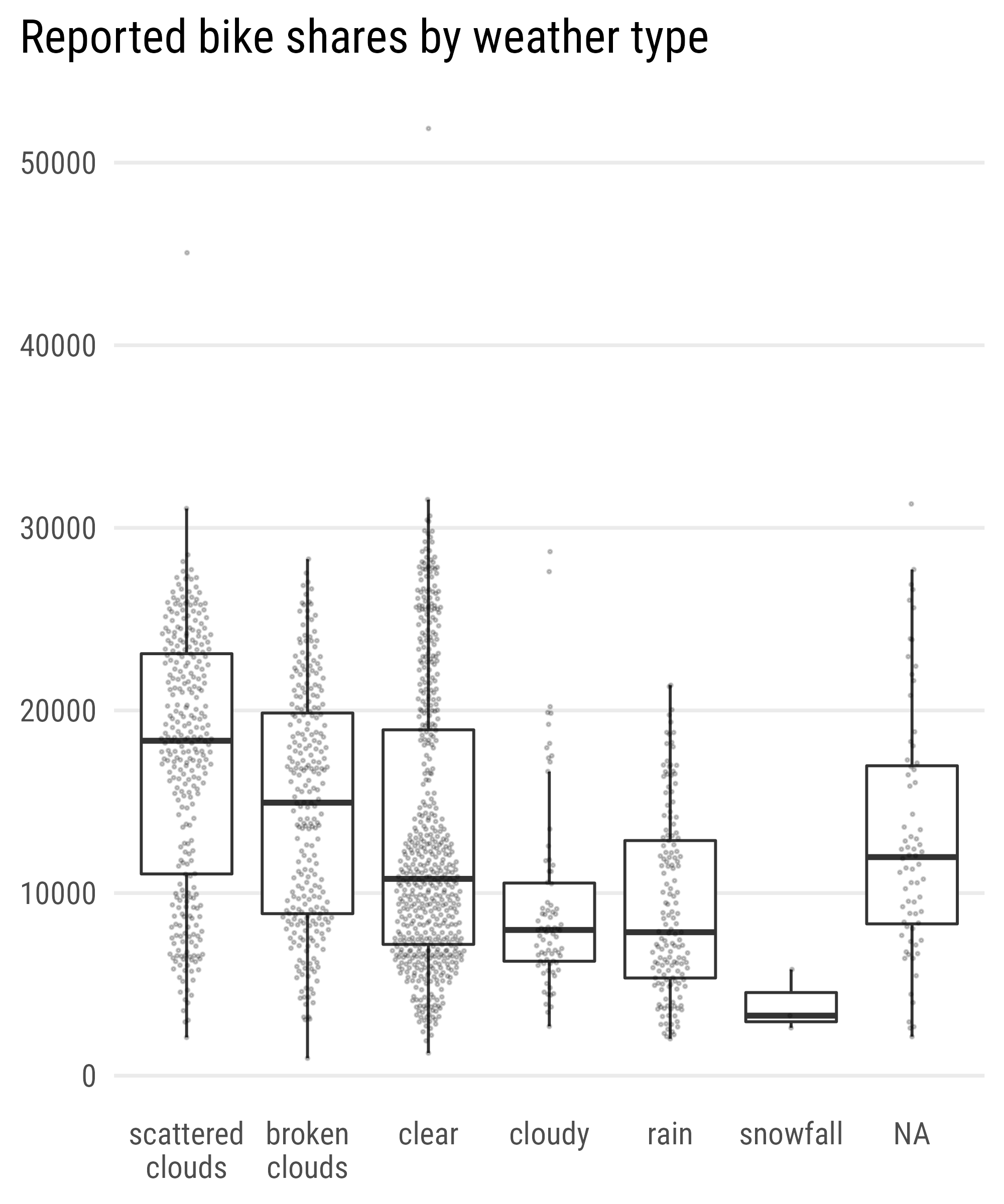
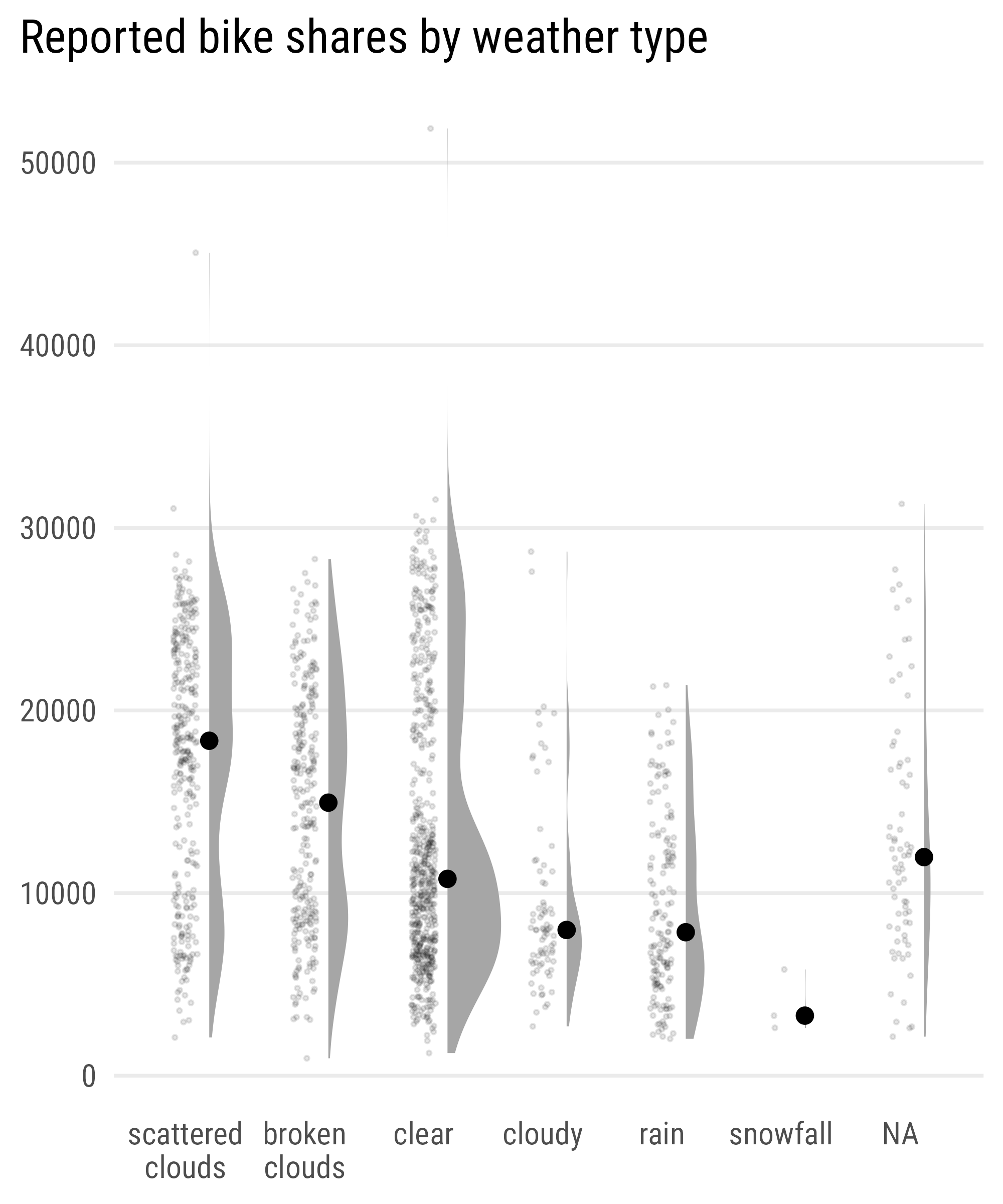
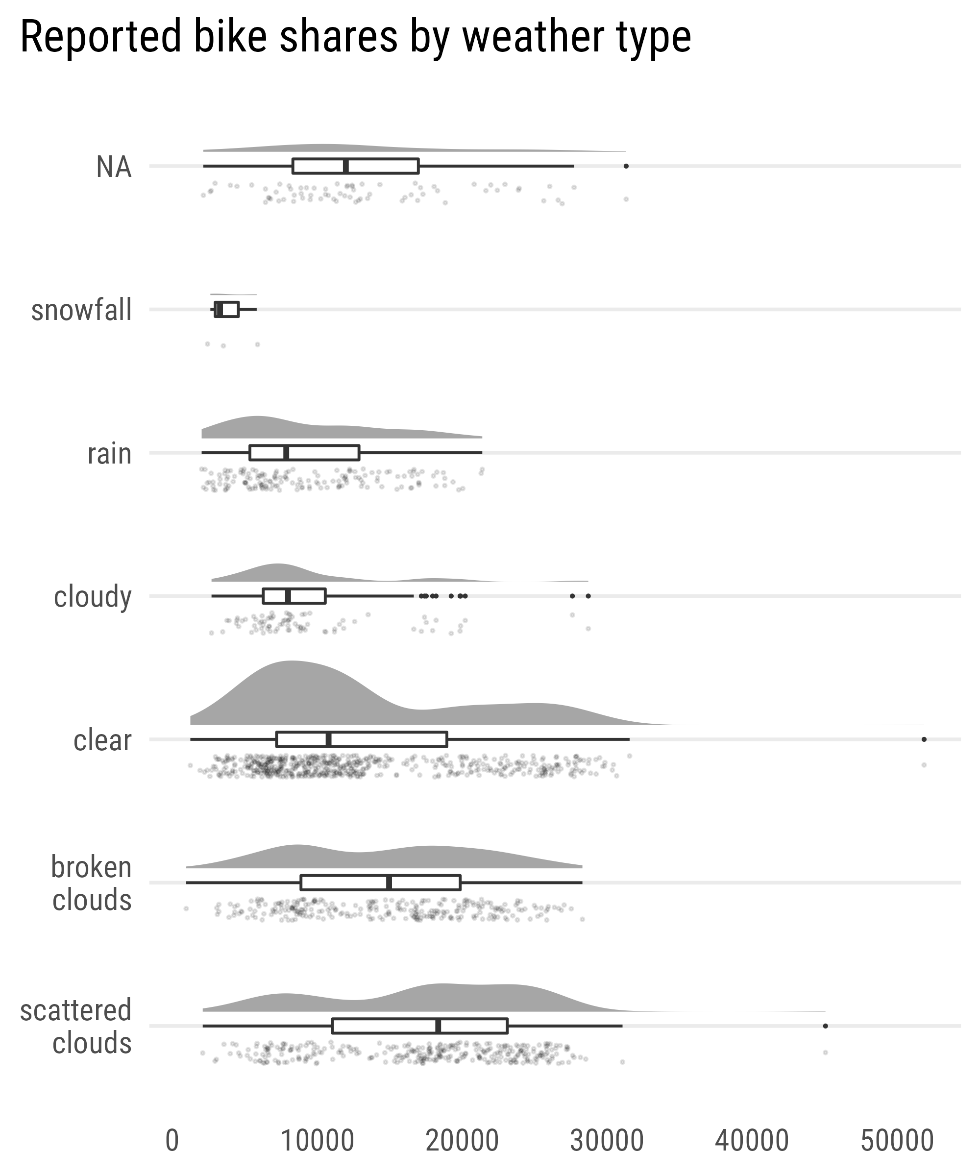
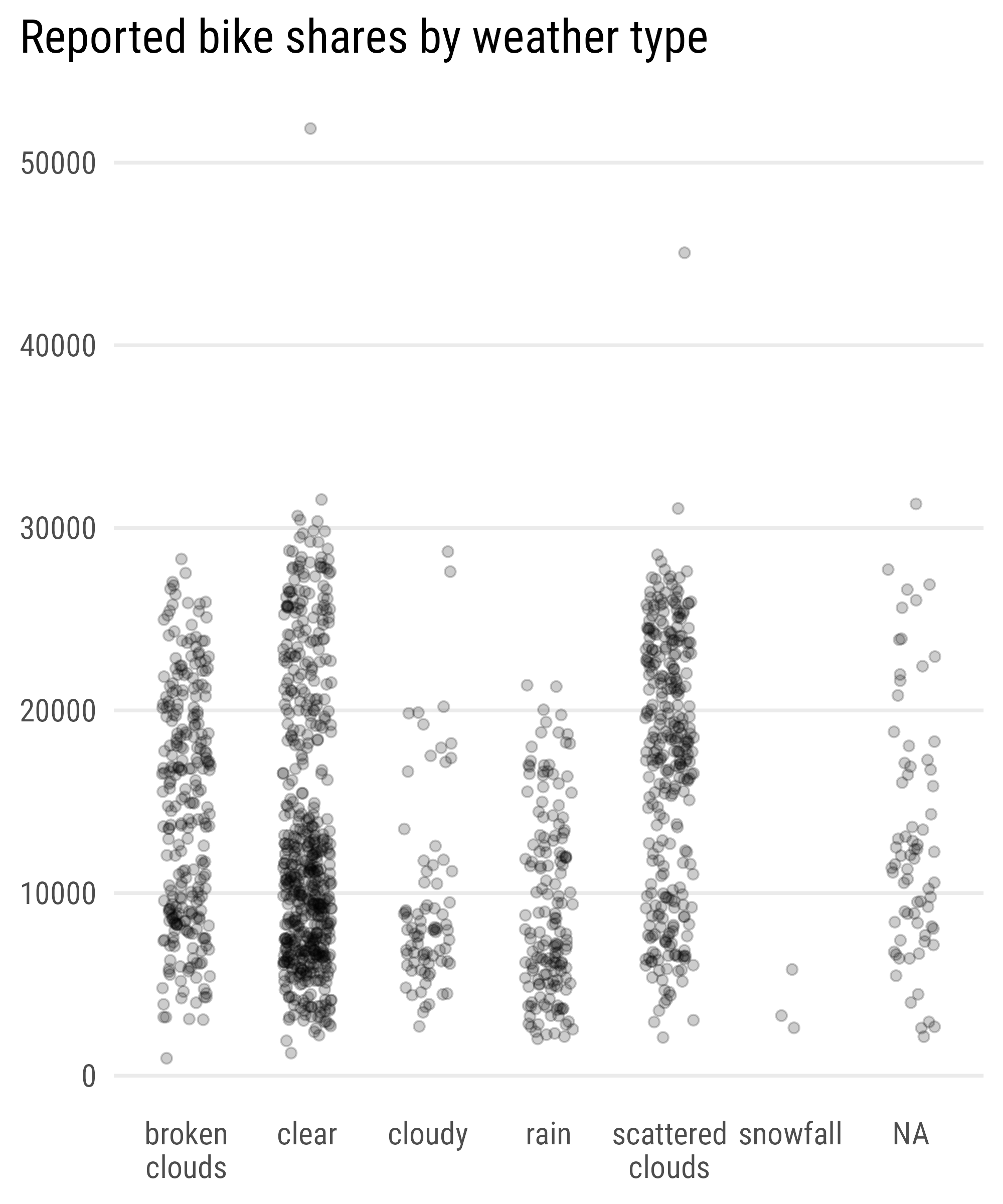
Jitter Strips of Counts per Weather Type
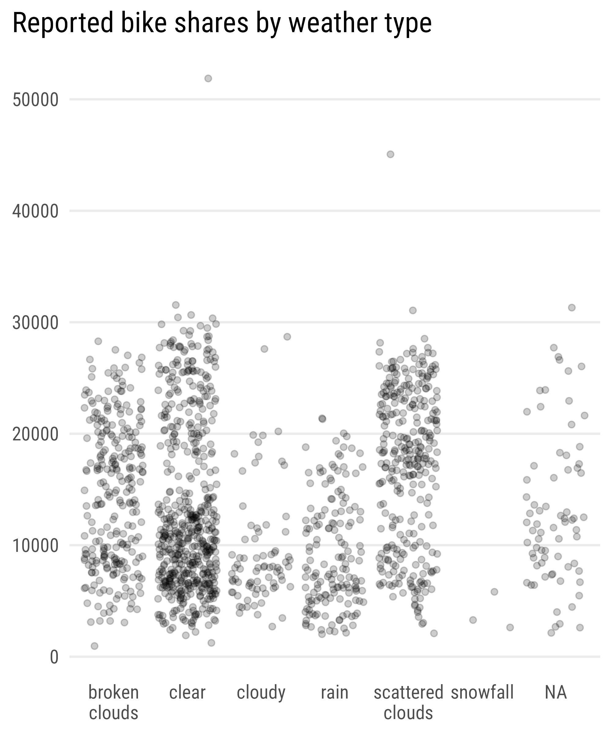
Jitter Strips of Counts per Weather Type

Jitter Strips of Counts vs. Weather Type
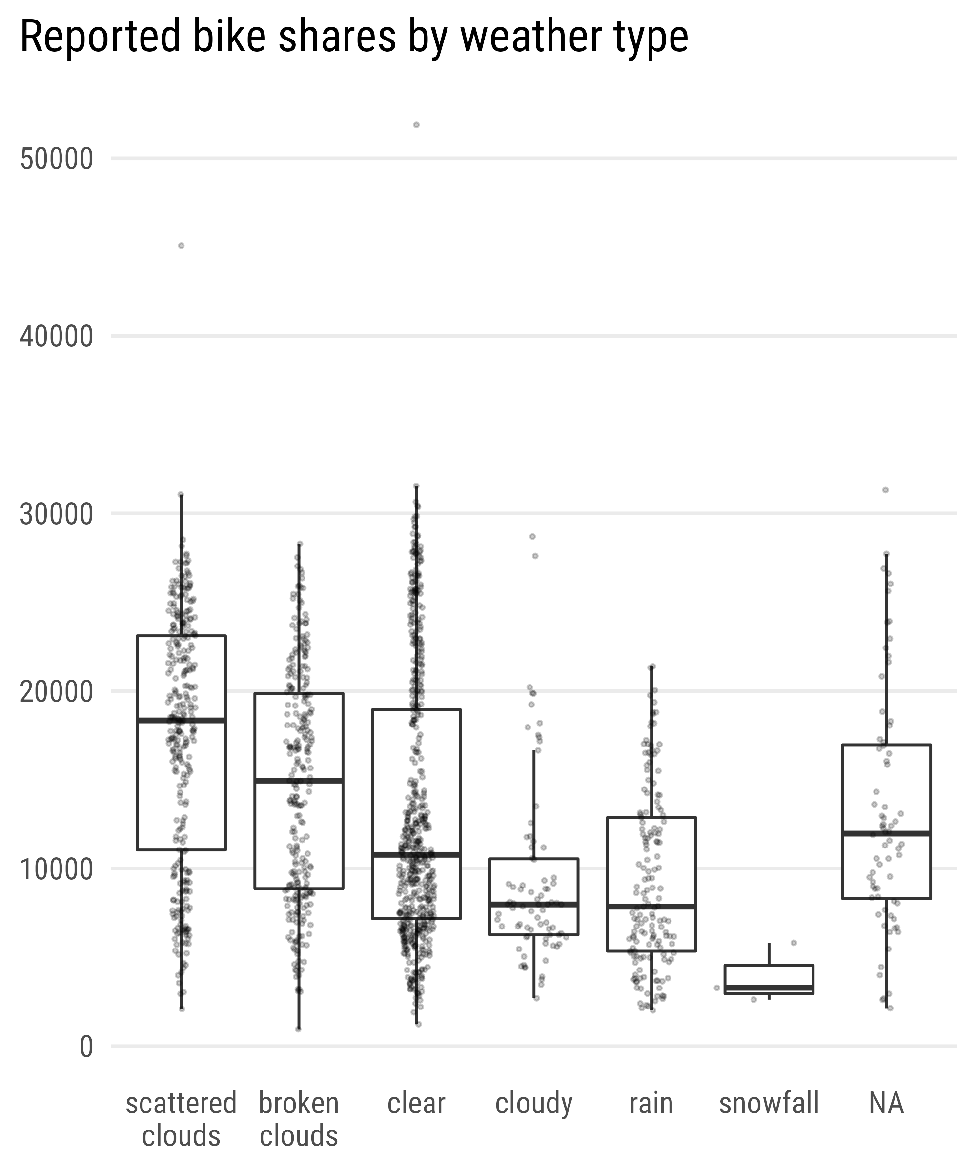
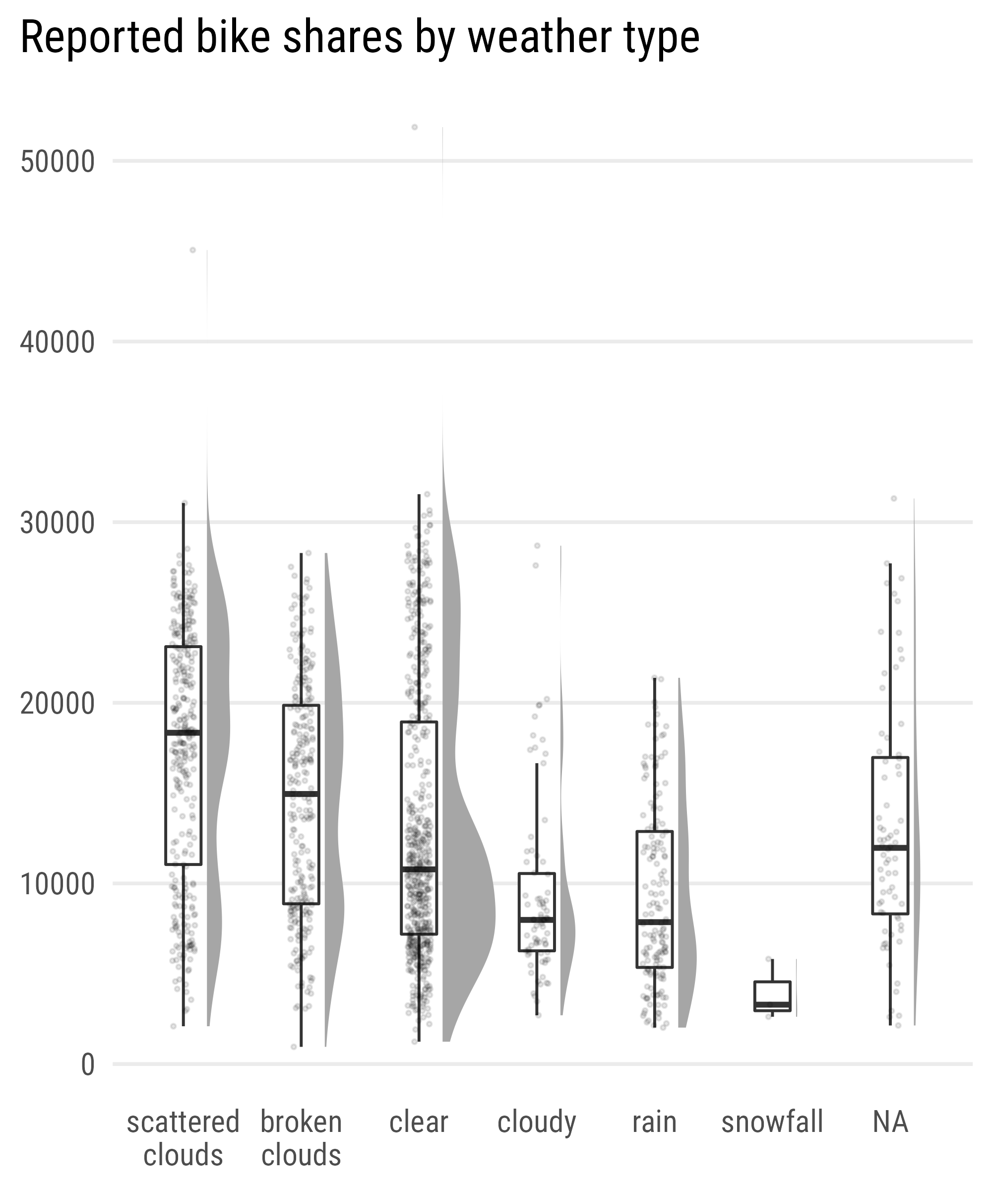
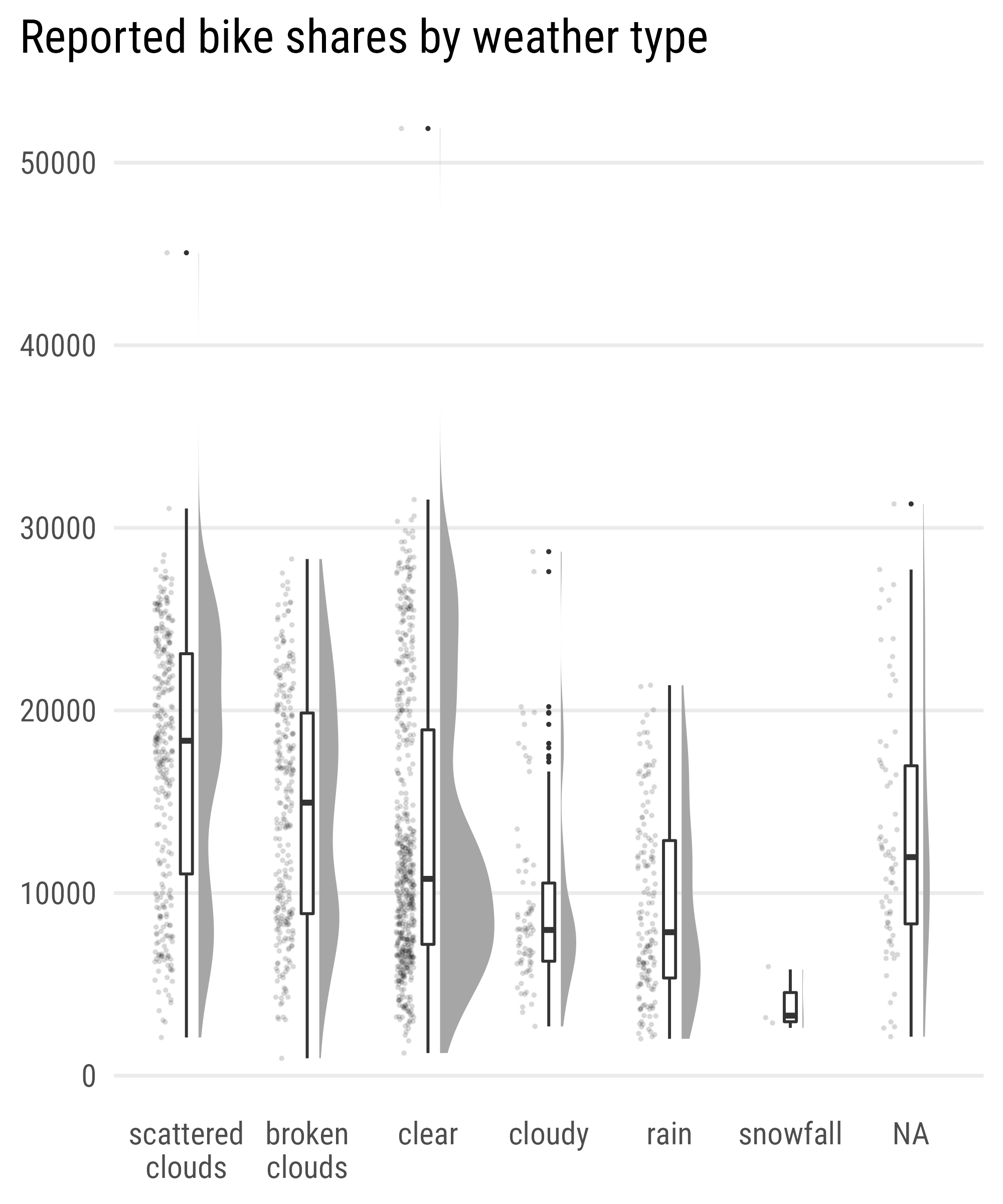
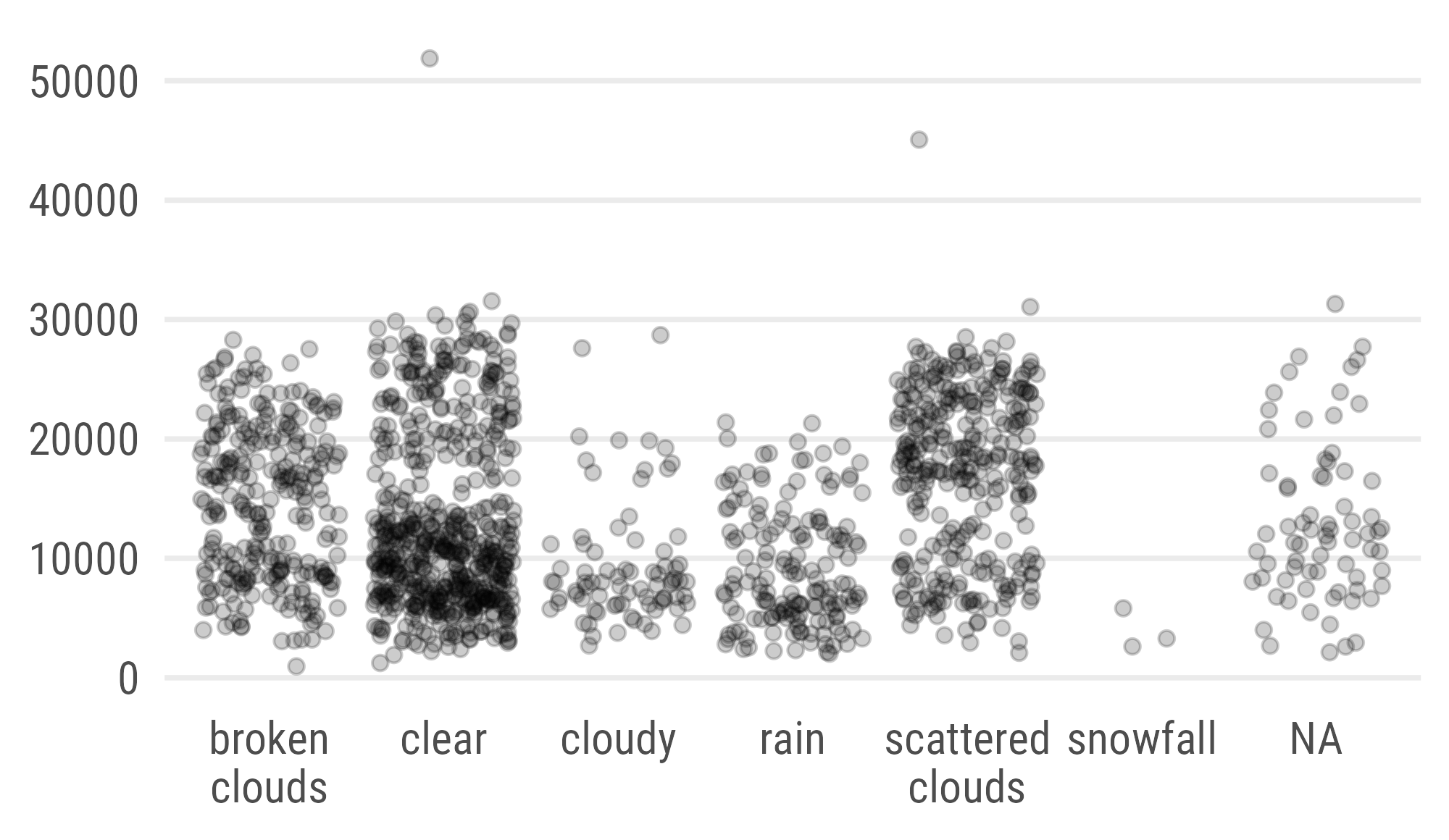
Boxplot + Jitter Strip Hybrid
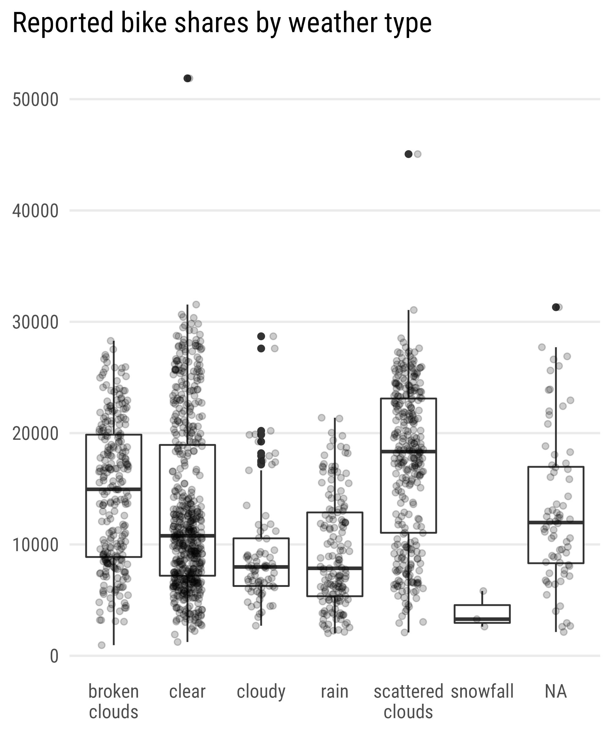
Boxplot + Jitter Strip Hybrid

Bonus: Sort Weather Types
ggplot(
bikes,
aes(
x = forcats::fct_reorder(
str_wrap(weather_type, 6), -count
),
y = count)
) +
geom_boxplot(
outlier.shape = NA
# outlier.color = "transparent"
# outlier.alpha = 0
) +
geom_point(
position = position_jitter(
seed = 2022,
width = .2,
height = 0
),
alpha = .2
) +
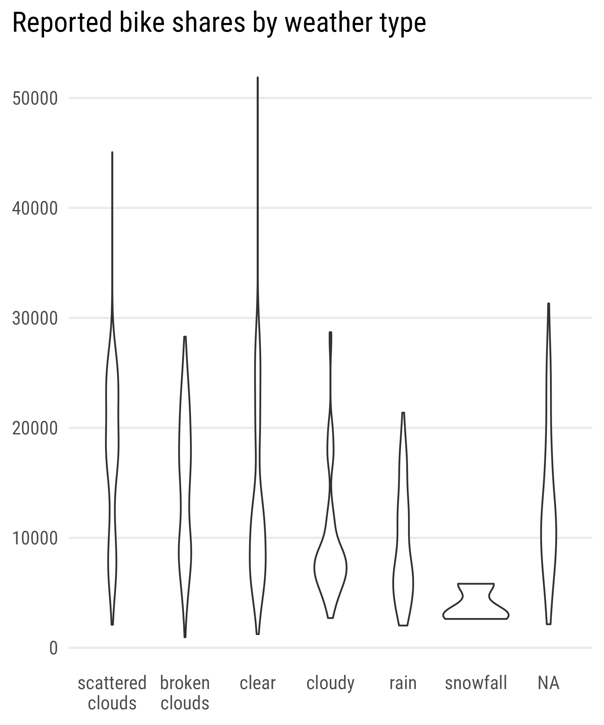
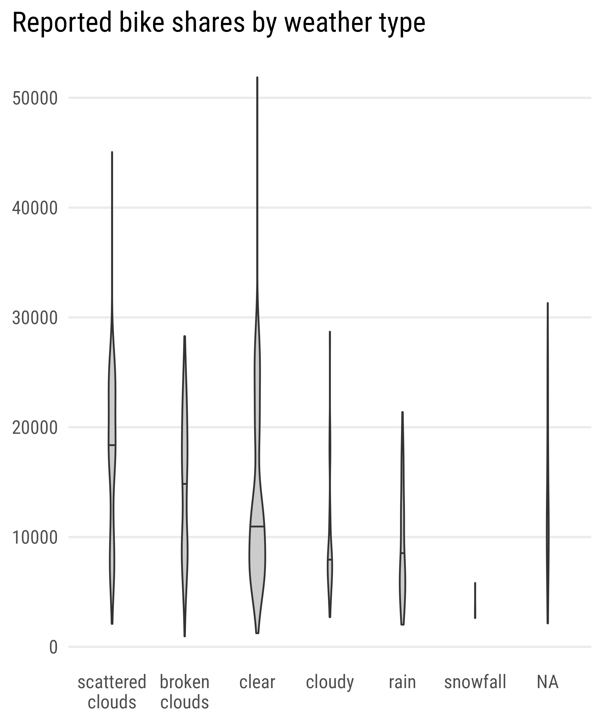
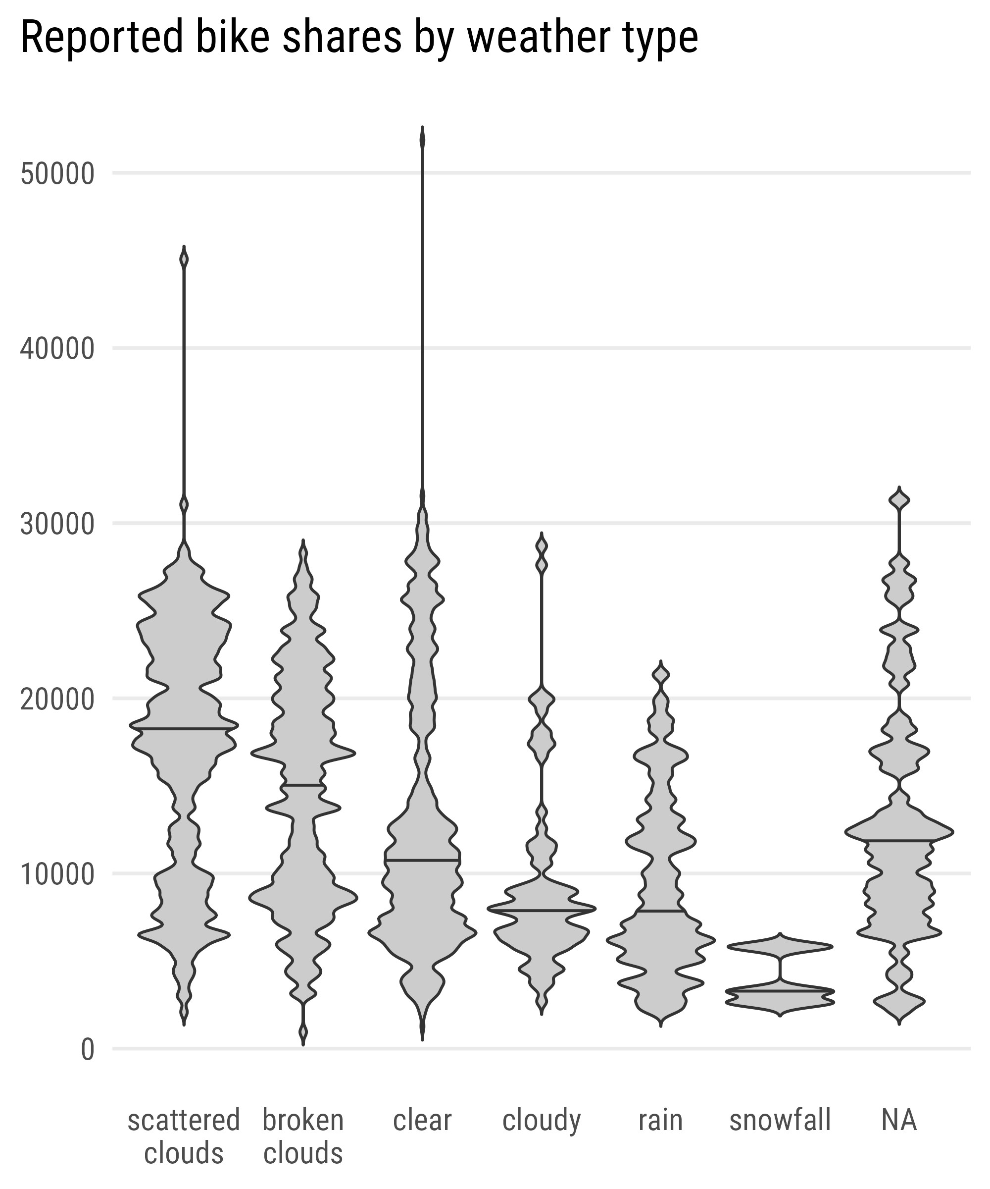
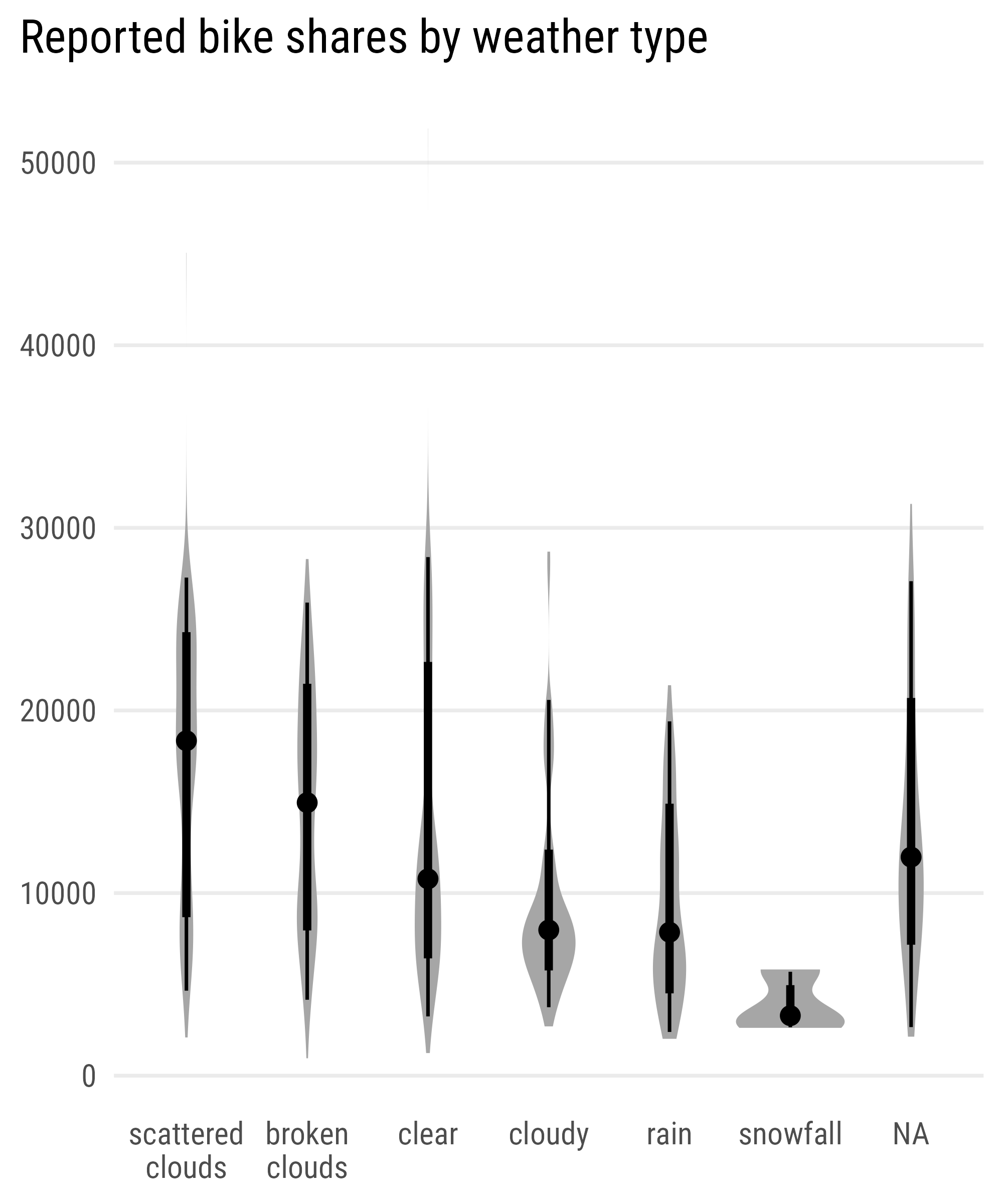
ggtitle("Reported bike shares by weather type")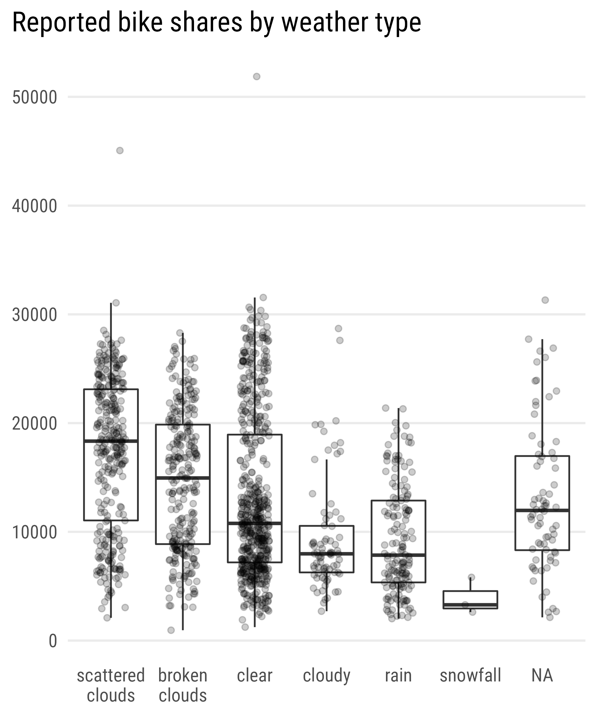
Save the Plot