library(tidyverse)

df_astro <- readr::read_csv(
  'https://raw.githubusercontent.com/rfordatascience/tidytuesday/master/data/2020/2020-07-14/astronauts.csv'
)

df_missions <-
  df_astro %>%
  group_by(name) %>%
  summarize(
    hours = sum(hours_mission),
    year = min(year_of_mission),
    max_year = max(year_of_mission)
  ) %>%
  ungroup() %>%
  mutate(year = -year) %>%
  arrange(year) %>%
mutate(id = row_number())Graphic Design with ggplot2
Concepts of the {ggplot2} Package Pt. 2:
Solution Exercise 1
Cédric Scherer // rstudio::conf // July 2022
Exercise 1
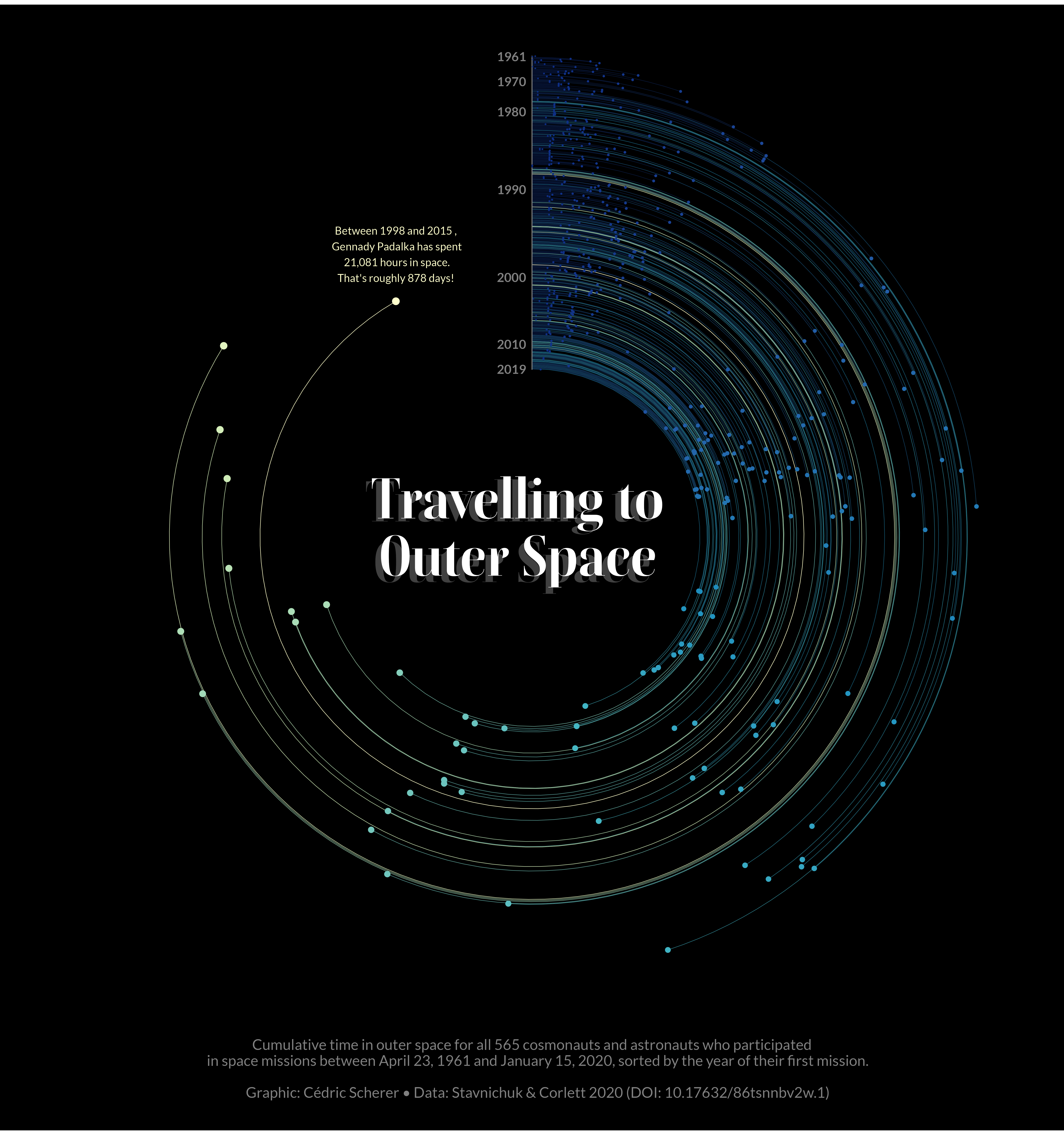
- Have a look at the following visualization of the cumulative time that cosmo- and astronauts have spent in outer space. The data also contains information on the year of their first and last travel, respectively.
- Together with your group, discuss which layers and modifications are needed to create such a chart with
{ggplot2}.- Note down the aesthetics, geometries, and scales used for each element of this graphic.
- What is the coordinate system? Have any adjustments been made?
- Which theme was used and how was it modified?
Layers
geom_point()aes(x = id, y = hours, size = hours)
geom_linerange()aes(x = id, ymin = 0, ymax = hours, color = hours, alpha = hours)
geom_point()aes(x = id, y = 0), shape = 15, color = "#808080"
geom_text()aes(x = id, y = 0, label = year), size = 4.5, hjust = 1.2
geom_text()aes(x = id, y = hours, label = max), size = 3.9, vjust = -.35
Scales
scale_x_continuous()limits = c(-300, NA), expand = c(0, 0)
scale_y_continuous()limits = c(0, 230000), expand = c(0, 0)
scale_color_distiller()palette = "YlGnBu, direction = -1
scale_size()range = c(.001, 3)
scale_alpha()range = c(.33, .95)
Coordinate System
coord_polar()theta = "y"
Coordinate System
coord_polar()theta = "y"
Theme
theme_void()legend.position = "none"plot.background = element_rect(fill = "black")plot.margin = margin(-70, -70, -70, -70)plot.caption = element_text(hjust = .5, margin = margin(-100, 0, 100, 0), ...)
Coordinate System
coord_polar()theta = "y"
Theme
theme_void()legend.position = "none"plot.background = element_rect(fill = "black")plot.margin = margin(-70, -70, -70, -70)plot.caption = element_text(...)
Title
- 2 x
annotate(geom = "text", x = -300, y = 0, ...)
Data Prep
Code Pt. 1
# install.packages("scico")

g1 <-
  ggplot(df_missions, aes(x = id, y = hours, color = hours)
    ) +
    ## curves
    geom_linerange(aes(ymin = 0, ymax = hours, alpha = hours), size = .25) +
    ## baseline
    geom_point(aes(y = 0), shape = 15, size = .1, color = "#808080") +
    ## points
    geom_point(aes(y = hours, size = hours)) +
    ## turn into circular
    coord_polar(theta = "y", start = 0, clip = "off") +
    ## add axis spacings
    scale_x_continuous(limits = c(-300, NA), expand = c(0, 0)) +
    scale_y_continuous(limits = c(0, 23000), expand = c(0, 0)) +
    ## change colors, transparencies, and bubble sizes
    scale_color_distiller(palette = "YlGnBu", direction = -1) +
    scale_size(range = c(.001, 3)) +
    scale_alpha(range = c(.33, .95)) +
    ## remove all theme components
    theme_void() +
    theme(
      ## set dark background
      plot.background = element_rect(fill = "black"),
      ## remove "white" space
      plot.margin = margin(-70, -70, -70, -70),
      ## remove legends
      legend.position = "none"
    )
Data Prep Labels
df_labs <-
  df_missions %>%
  filter(year %in% -c(1961, 197:201*10, 2019)) %>%
  group_by(year) %>%
  filter(id == min(id))

df_max <-
  df_missions %>%
  arrange(-hours) %>%
  slice(1) %>%
  mutate(
    first_name = str_remove(name, ".*, "),
    last_name = str_remove(name, "(?<=),.*"),
    label = paste("Between", abs(year), "and", max_year, ",\n", first_name, last_name, "has spent\n", format(hours, big.mark = ','), "hours in space.\nThat's roughly", round(hours / 24, 0), "days!")
  )
Code Pt. 2
g2 <-
  g1 +
    ## labels years
    geom_text(
      data = df_labs, aes(y = 0, label = abs(year)),
      family = "Lato", fontface = "bold", color = "#808080",
      size = 4.5, hjust = 1.2
    ) +
    ## label max
    geom_text(
      data = df_max, aes(label = label),
      family = "Lato", size = 3.9, vjust = -.35
    ) +
    ## title shadow
    annotate(
      geom = "text", x = -300, y = 0, label = "Travelling to\nOuter Space",
      family = "Boska", fontface = "bold", lineheight = .9,
      size = 20, color = "white", hjust = .57, vjust = .45, alpha = .25
    ) +
    ## title
    annotate(
      geom = "text", x = -300, y = 0, label = "Travelling to\nOuter Space",
      family = "Boska", fontface = "bold", lineheight = .85,
      size = 20, color = "white", hjust = .55, vjust = .4
    ) +
    ## caption
    labs(caption = "Cumulative time in outer space for all 565 cosmonauts and astronauts who participated
    in space missions between April 23, 1961 and January 15, 2020, sorted by the year of their first mission.

    Graphic: Cédric Scherer • Data: Stavnichuk & Corlett 2020 (DOI: 10.17632/86tsnnbv2w.1)") +
    ## modify caption + move inside plot area
    theme(
      plot.caption = element_text(
        family = "Lato",
        size = 15, color = "#808080", hjust = .5,
        margin = margin(-100, 0, 100, 0)
      )
    )
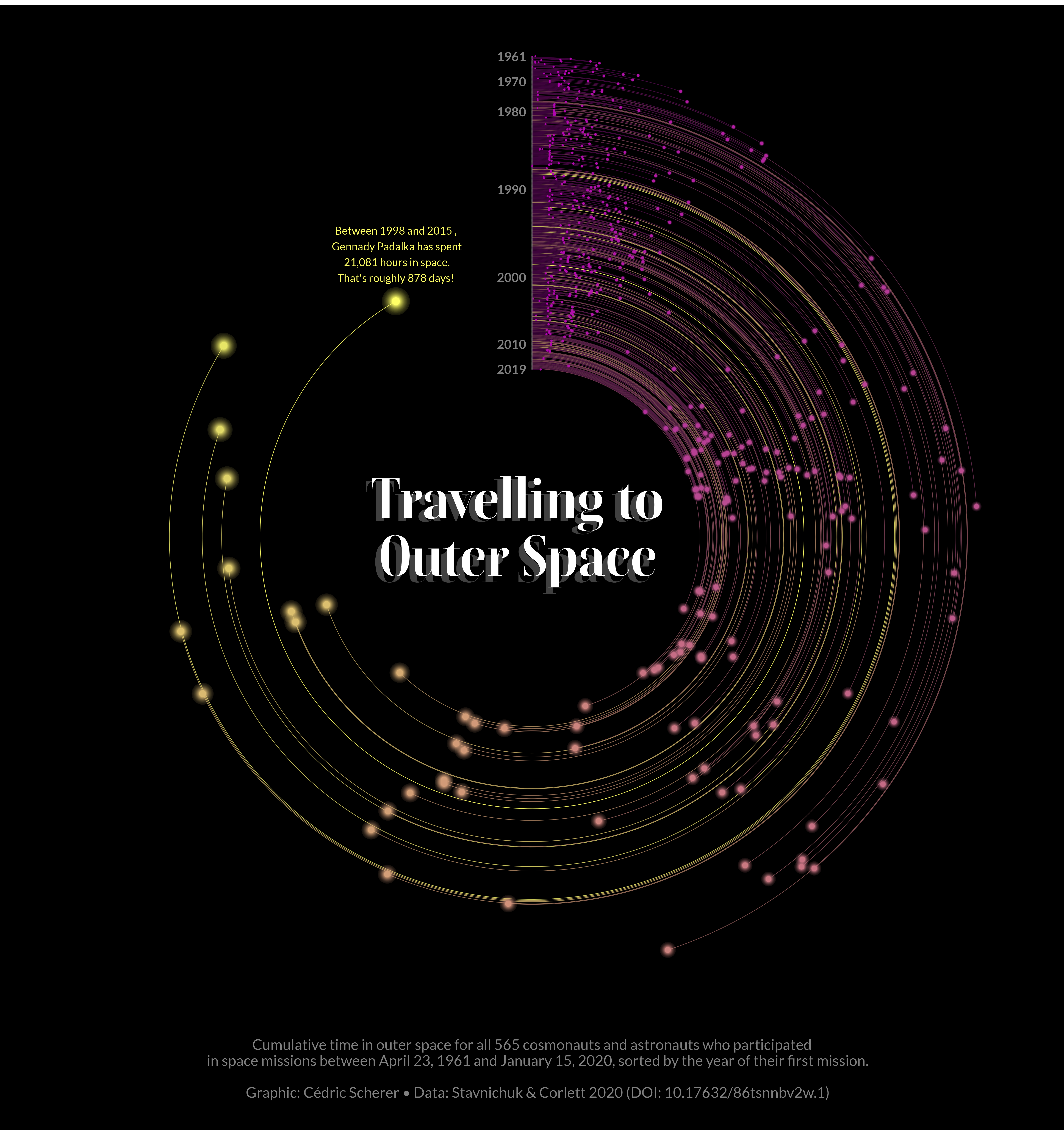
Code with Special Extensions
# install.packages("ggforce")
# install.packages("scico")
# devtools::install_github("coolbutuseless/ggblur")

g_ext <-
  ggplot(df_missions, aes(x = id, y = hours, color = hours)) +
    ## geom_link() from {ggforce} to draw smooth curves
    ggforce::geom_link(aes(xend = id, yend = 0, alpha = hours), size = .25, n = 300) +
    geom_point(aes(y = 0), shape = 15, size = .1, color = "#808080") +
    ##geom_point_blur() from {ggblur} to add points with gradual fading
    ggblur::geom_point_blur(aes(size = hours, blur_size = hours), blur_steps = 25) +
    geom_text(
      data = df_labs, aes(y = 0, label = abs(year)),
      family = "Lato", fontface = "bold", color = "#808080",
      size = 4.5, hjust = 1.2
    ) +
    geom_text(
      data = df_max, aes(label = label),
      family = "Lato", size = 3.9, vjust = -.35
    ) +
    coord_polar(theta = "y", start = 0, clip = "off") +
    scale_x_continuous(limits = c(-300, NA), expand = c(0, 0)) +
    scale_y_continuous(limits = c(0, 23000), expand = c(0, 0)) +
    ## use custom color palette from {scico}
    scico::scale_color_scico(palette = "buda") +
    scale_size(range = c(.001, 3)) +
    ggblur::scale_blur_size_continuous(range = c(.5, 10), guide = "none") +
    scale_alpha(range = c(.33, .95)) +
    annotate(
      geom = "text", x = -300, y = 0, label = "Travelling to\nOuter Space",
      family = "Boska", fontface = "bold", lineheight = .9,
      size = 20, color = "white", hjust = .57, vjust = .45, alpha = .25
    ) +
    annotate(
      geom = "text", x = -300, y = 0, label = "Travelling to\nOuter Space",
      family = "Boska", fontface = "bold", lineheight = .85,
      size = 20, color = "white", hjust = .55, vjust = .4
    ) +
    labs(caption = "Cumulative time in outer space for all 565 cosmonauts and astronauts who participated
    in space missions between April 23, 1961 and January 15, 2020, sorted by the year of their first mission.

    Graphic: Cédric Scherer • Data: Stavnichuk & Corlett 2020 (DOI: 10.17632/86tsnnbv2w.1)") +
    theme_void() +
    theme(
      plot.background = element_rect(fill = "black"),
      plot.margin = margin(-70, -70, -70, -70),
      legend.position = "none",
      plot.caption = element_text(
        family = "Lato",
        size = 15, color = "#808080", hjust = .5,
        margin = margin(-100, 0, 100, 0)
      )
    )
Cédric Scherer // rstudio::conf // July 2022