Graphic Design with ggplot2

Concepts of the {ggplot2} Package Pt. 2:
Solution Exercise 2

Cédric Scherer // rstudio::conf // July 2022

Exercise 2

• Create a circular lollipop plot of reported bike shares per season.
  • The data is not in the right format as there are no totals.
    How can you solve it?
  • Remove all legend elements (with a single line of code).
  • How can you add the labels next to the starting point of each lollipop?
  • How could you add a baseline?

Preparation

library(tidyverse)

bikes <- readr::read_csv(
  here::here("data", "london-bikes-custom.csv"),
  col_types = "Dcfffilllddddc"
)

bikes$season <- stringr::str_to_title(bikes$season)
bikes$season <- forcats::fct_inorder(bikes$season)

theme_set(theme_light(base_size = 14, base_family = "Roboto Condensed"))

Lollipop Plot with Pre-Calculated Sums

bikes %>%
  group_by(season) %>%
  summarize(count = sum(count))

# A tibble: 4 x 2
  season   count
  <fct>    <int>
1 Winter 3520407
2 Spring 4850236
3 Summer 6424609
4 Autumn 5073040

Lollipop Plot with Pre-Calculated Sums

bikes %>%
  group_by(season) %>%
  summarize(count = sum(count)) %>%
  ggplot(aes(x = season, y = count)) +
  geom_point(size = 3) +
  geom_linerange(
    aes(ymin = 0, ymax = count)
  )

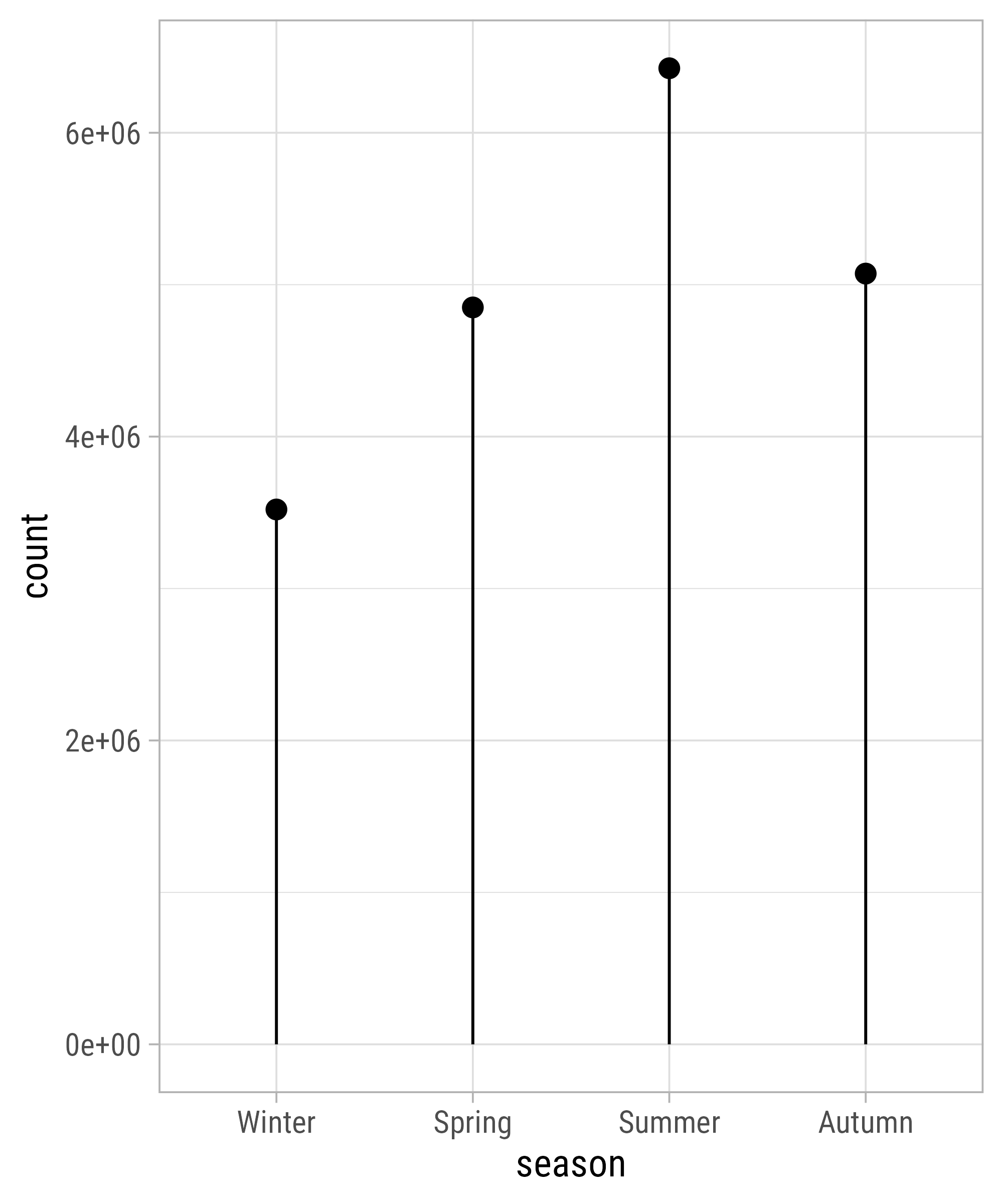
Calculate Sums via stat_summary()

ggplot(bikes, aes(x = season, y = count)) +
  stat_summary(
    geom = "point", fun = "sum", size = 3
  ) +
  stat_summary(
    geom = "linerange", ymin = 0,
    fun.max = function(y) sum(y)
  )

Calculate Sums via stat_summary()

ggplot(bikes, aes(x = season, y = count)) +
  stat_summary(
    geom = "point", fun = "sum", size = 3
  ) +
  stat_summary(
    geom = "linerange", ymin = 0,
    fun.max = function(y) sum(y)
  ) +
  coord_cartesian(ylim = c(0, NA))

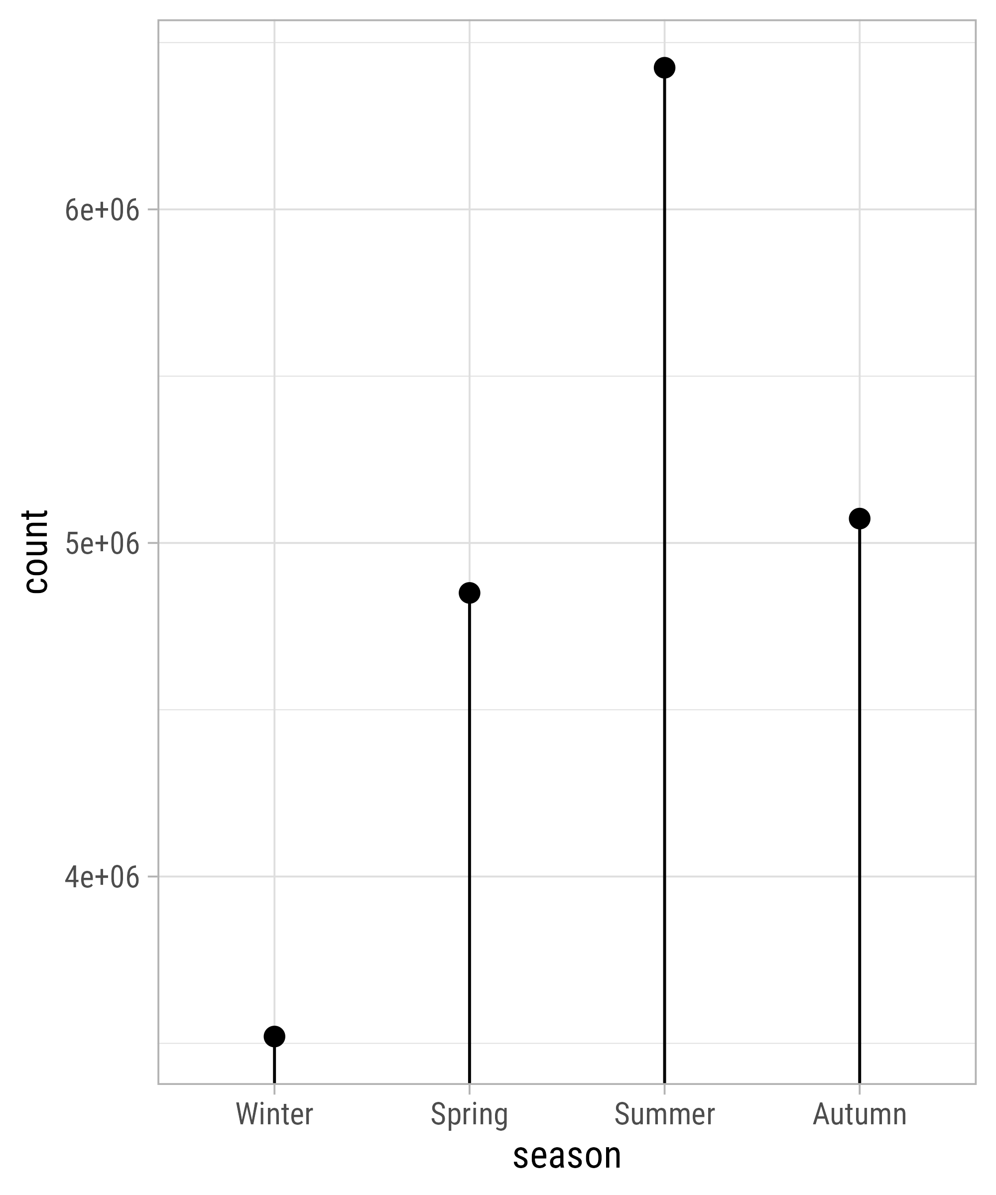
Apply a Polar Coordinate System

bikes %>%
  group_by(season) %>%
  summarize(count = sum(count)) %>%
  ggplot(aes(x = season, y = count)) +
  geom_point(size = 3) +
  geom_linerange(
    aes(ymin = 0, ymax = count)
  ) +
  coord_polar(theta = "y")

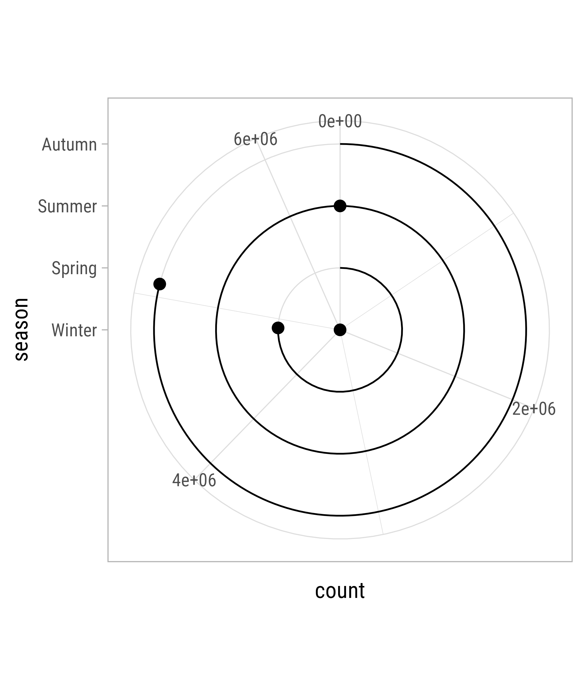
Fix Axis Ranges

bikes %>%
  group_by(season) %>%
  summarize(count = sum(count)) %>%
  ggplot(aes(x = season, y = count)) +
  geom_point(size = 3) +
  geom_linerange(
    aes(ymin = 0, ymax = count)
  ) +
  coord_polar(theta = "y") +
  scale_x_discrete(
    expand = c(.5, .5)
  ) +
  scale_y_continuous(
    limits = c(0, 7.5*10^6)
  )

Remove All Theme Components

bikes %>%
  group_by(season) %>%
  summarize(count = sum(count)) %>%
  ggplot(aes(x = season, y = count)) +
  geom_point(size = 3) +
  geom_linerange(
    aes(ymin = 0, ymax = count)
  ) +
  coord_polar(theta = "y") +
  scale_x_discrete(
    expand = c(.5, .5)
  ) +
  scale_y_continuous(
    limits = c(0, 7.5*10^6)
  ) +
  theme_void()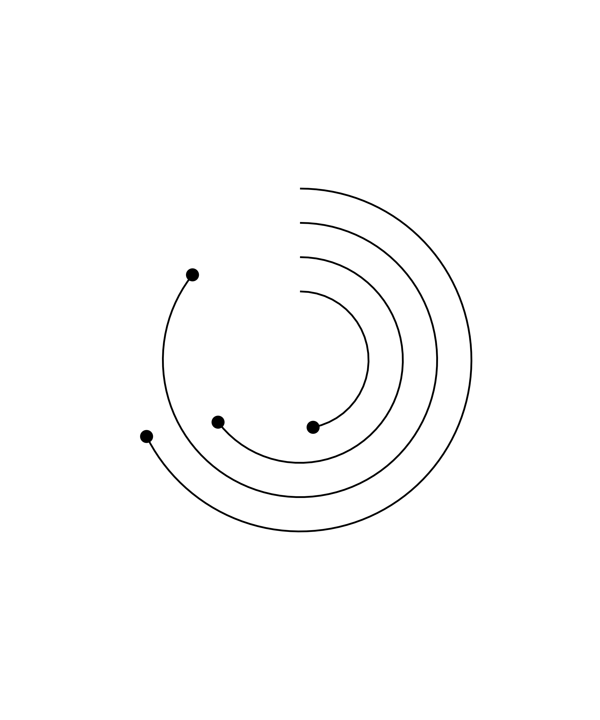

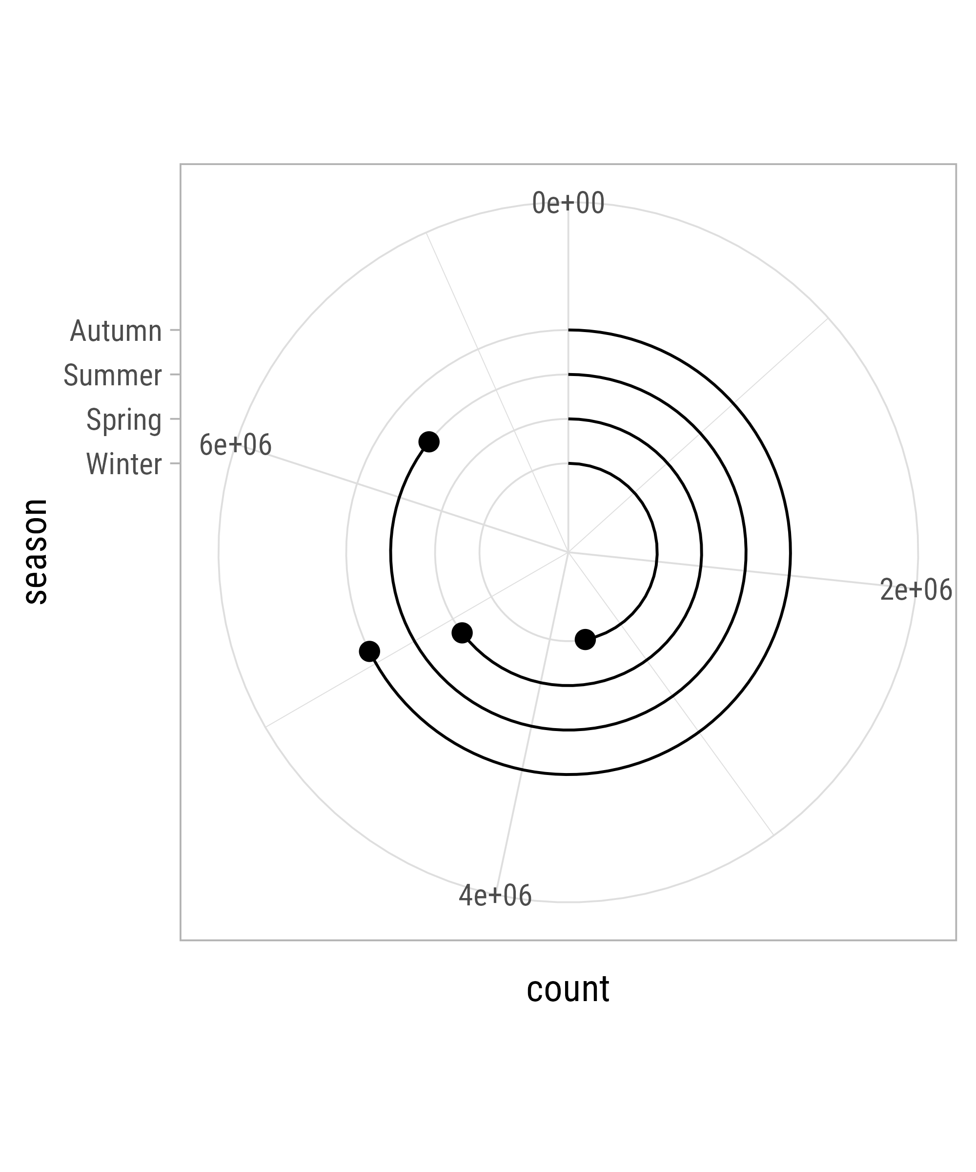
Fix Plot Margin

bikes %>%
  group_by(season) %>%
  summarize(count = sum(count)) %>%
  ggplot(aes(x = season, y = count)) +
  geom_point(size = 3) +
  geom_linerange(
    aes(ymin = 0, ymax = count)
  ) +
  coord_polar(theta = "y") +
  scale_x_discrete(
    expand = c(.5, .5)
  ) +
  scale_y_continuous(
    limits = c(0, 7.5*10^6)
  ) +
  theme_void() +
  theme(plot.margin = margin(rep(-100, 4)))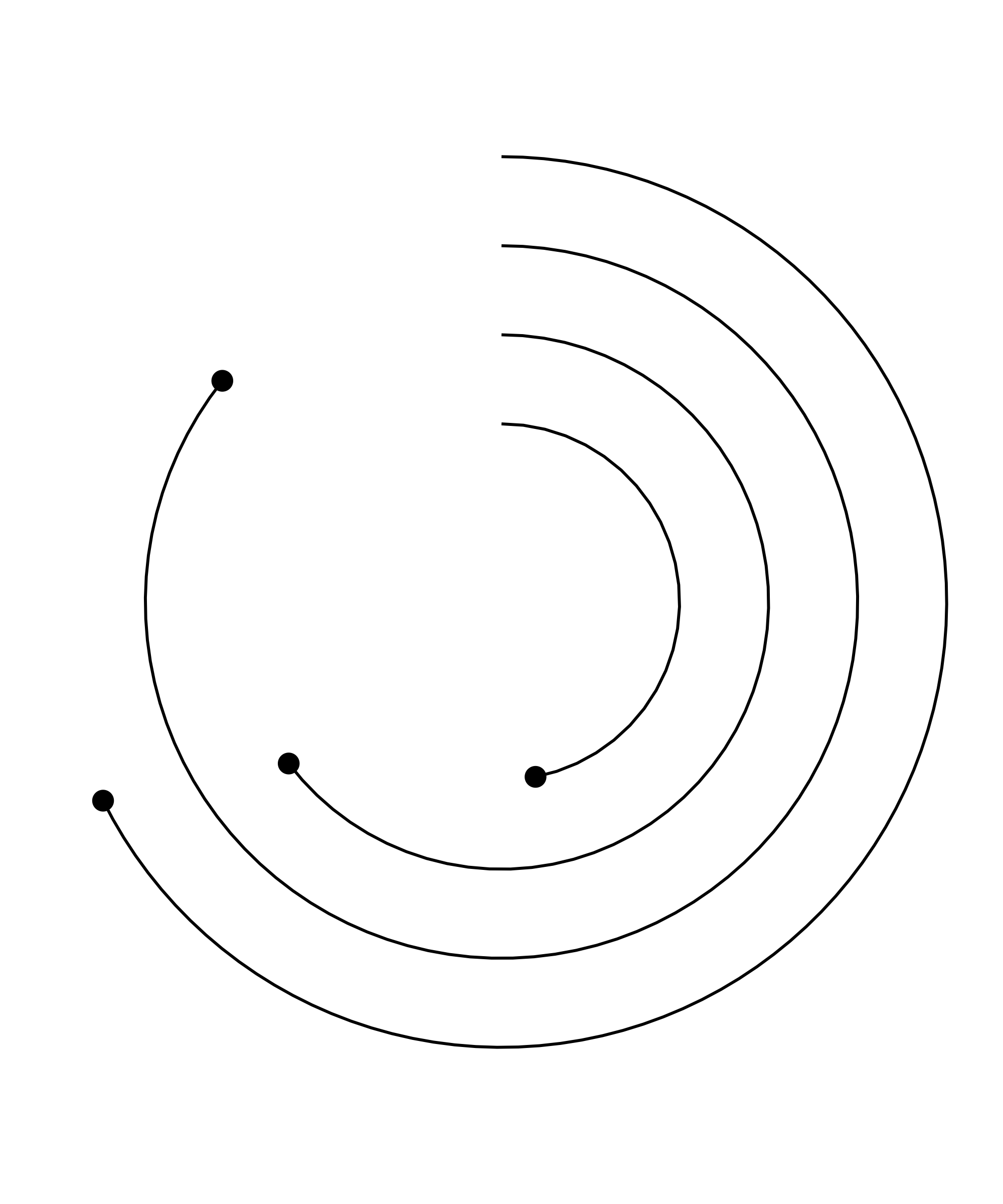

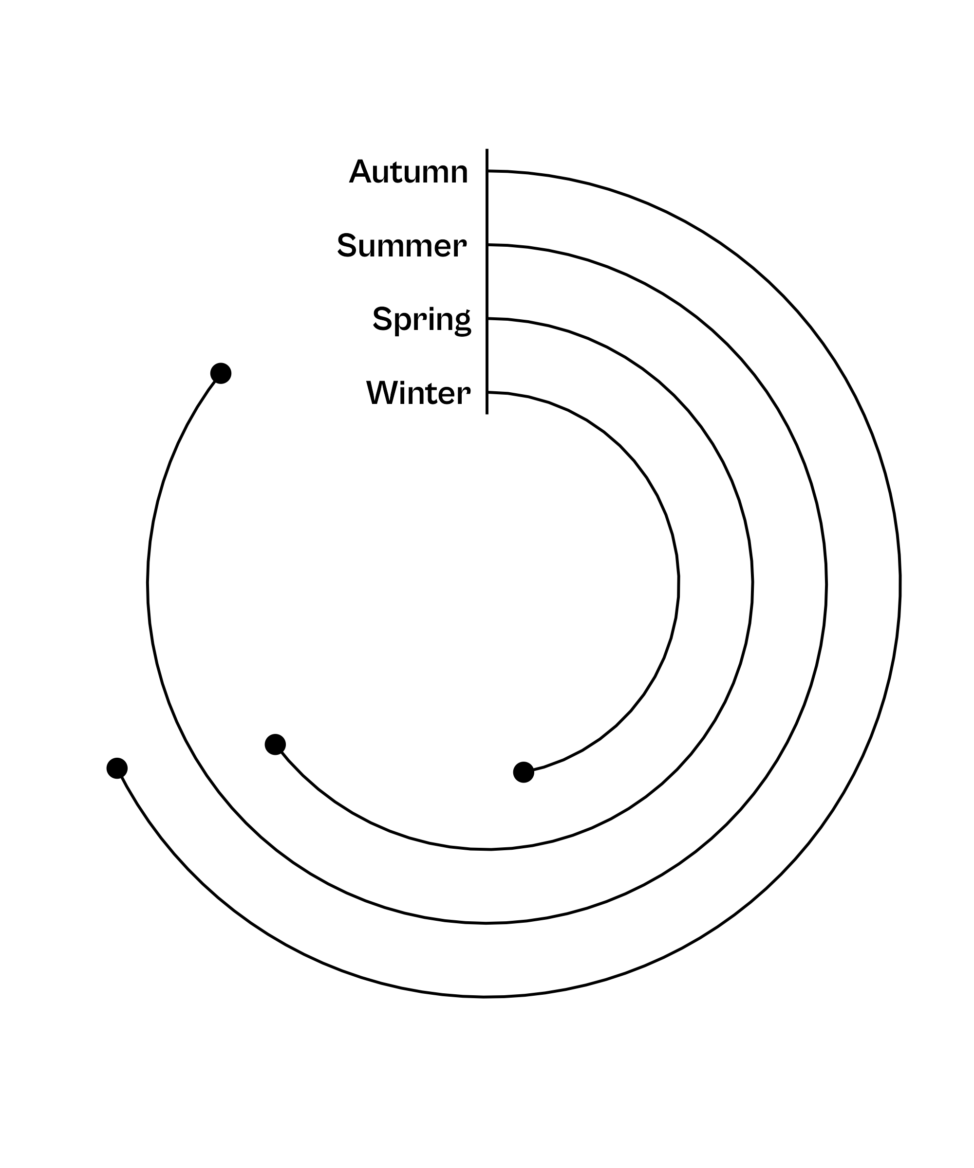
Add “Axis” Text

bikes %>%
  group_by(season) %>%
  summarize(count = sum(count)) %>%
  ggplot(aes(x = season, y = count)) +
  geom_point(size = 3) +
  geom_linerange(
    aes(ymin = 0, ymax = count)
  ) +
  geom_text(
    aes(label = season, y = 0)
  ) +
  coord_polar(theta = "y") +
  scale_x_discrete(
    expand = c(.5, .5)
  ) +
  scale_y_continuous(
    limits = c(0, 7.5*10^6)
  ) +
  theme_void() +
  theme(plot.margin = margin(rep(-100, 4)))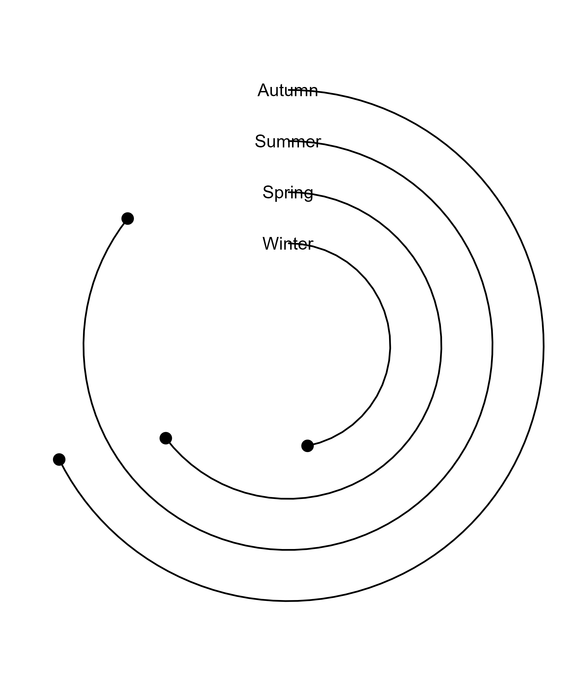

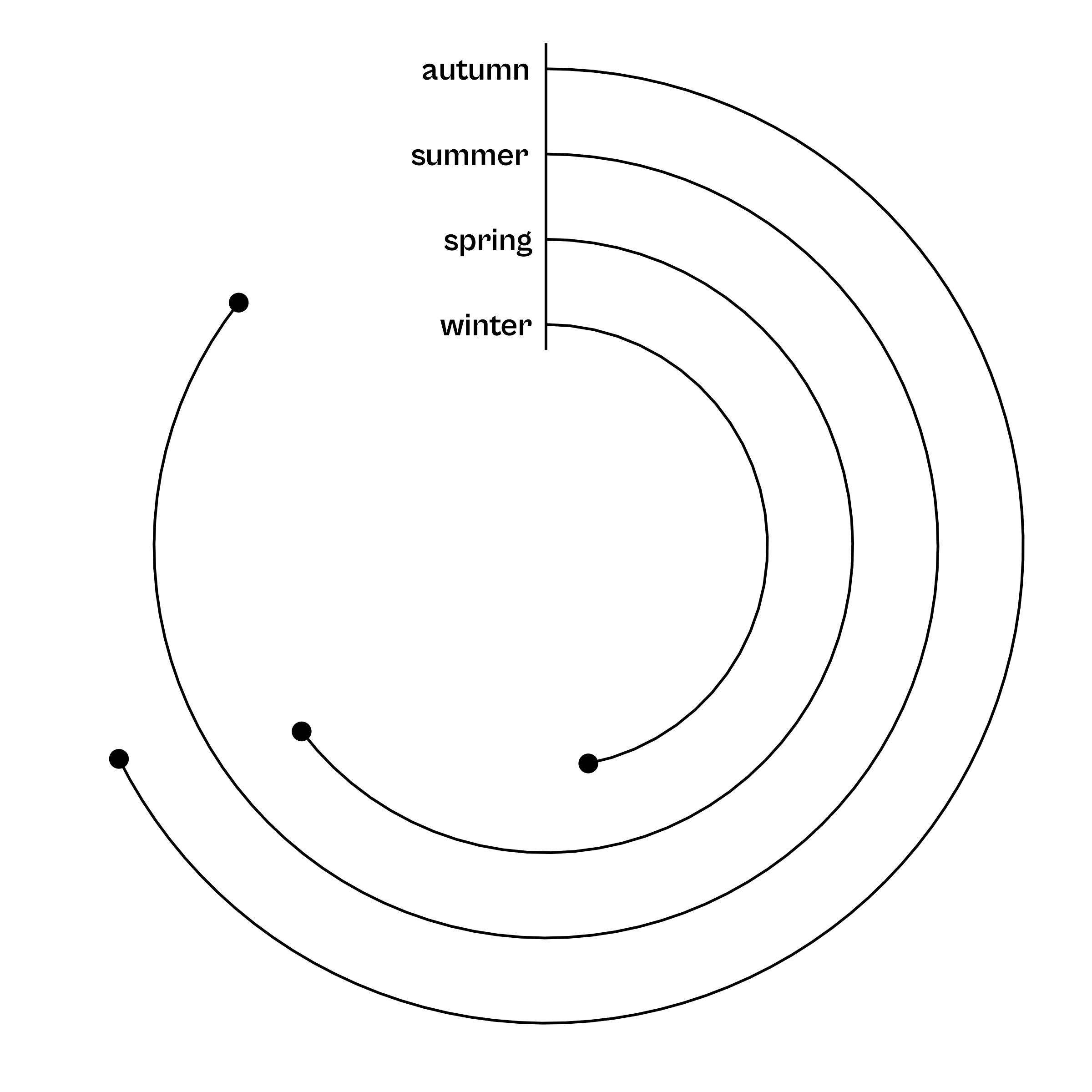
Style “Axis” Text

bikes %>%
  group_by(season) %>%
  summarize(count = sum(count)) %>%
  ggplot(aes(x = season, y = count)) +
  geom_point(size = 3) +
  geom_linerange(
    aes(ymin = 0, ymax = count)
  ) +
  geom_text(
    aes(label = season, y = 0),
    family = "Cabinet Grotesk", size = 4.5,
    fontface = "bold", hjust = 1.15
  ) +
  coord_polar(theta = "y") +
  scale_x_discrete(
    expand = c(.5, .5)
  ) +
  scale_y_continuous(
    limits = c(0, 7.5*10^6)
  ) +
  theme_void() +
  theme(plot.margin = margin(rep(-100, 4)))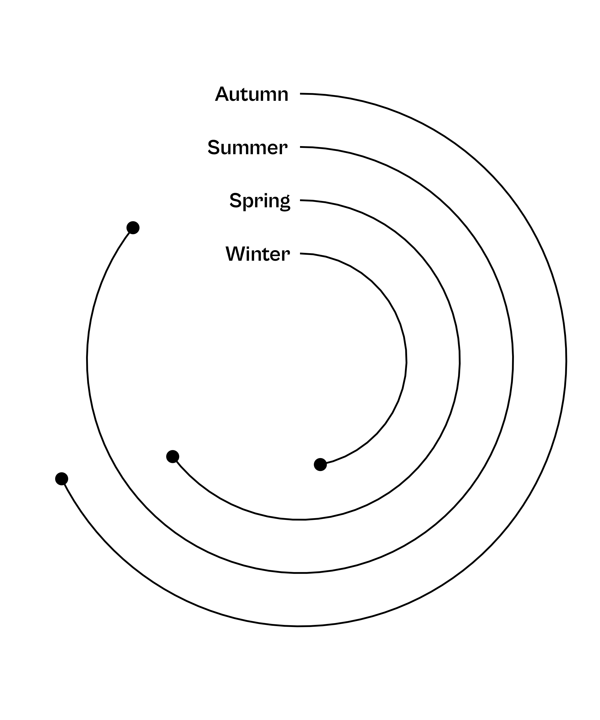

Alternatively: Add Direct Labels

bikes %>%
  group_by(season) %>%
  summarize(count = sum(count)) %>%
  ggplot(aes(x = season, y = count)) +
  geom_point(size = 3) +
  geom_linerange(
    aes(ymin = 0, ymax = count)
  ) +
  geom_text(
    aes(label = season, y = 0),
    family = "Cabinet Grotesk", size = 4.5,
    fontface = "bold", hjust = 1.15
  ) +
  geom_text(
    aes(label = paste0(round(count / 10^6, 1), "M")),
    size = 4, vjust = -1, family = "Cabinet Grotesk"
  ) +
  coord_polar(theta = "y") +
  scale_x_discrete(
    expand = c(.5, .5)
  ) +
  scale_y_continuous(
    limits = c(0, 7.5*10^6)
  ) +
  theme_void() +
  theme(plot.margin = margin(rep(-100, 4)))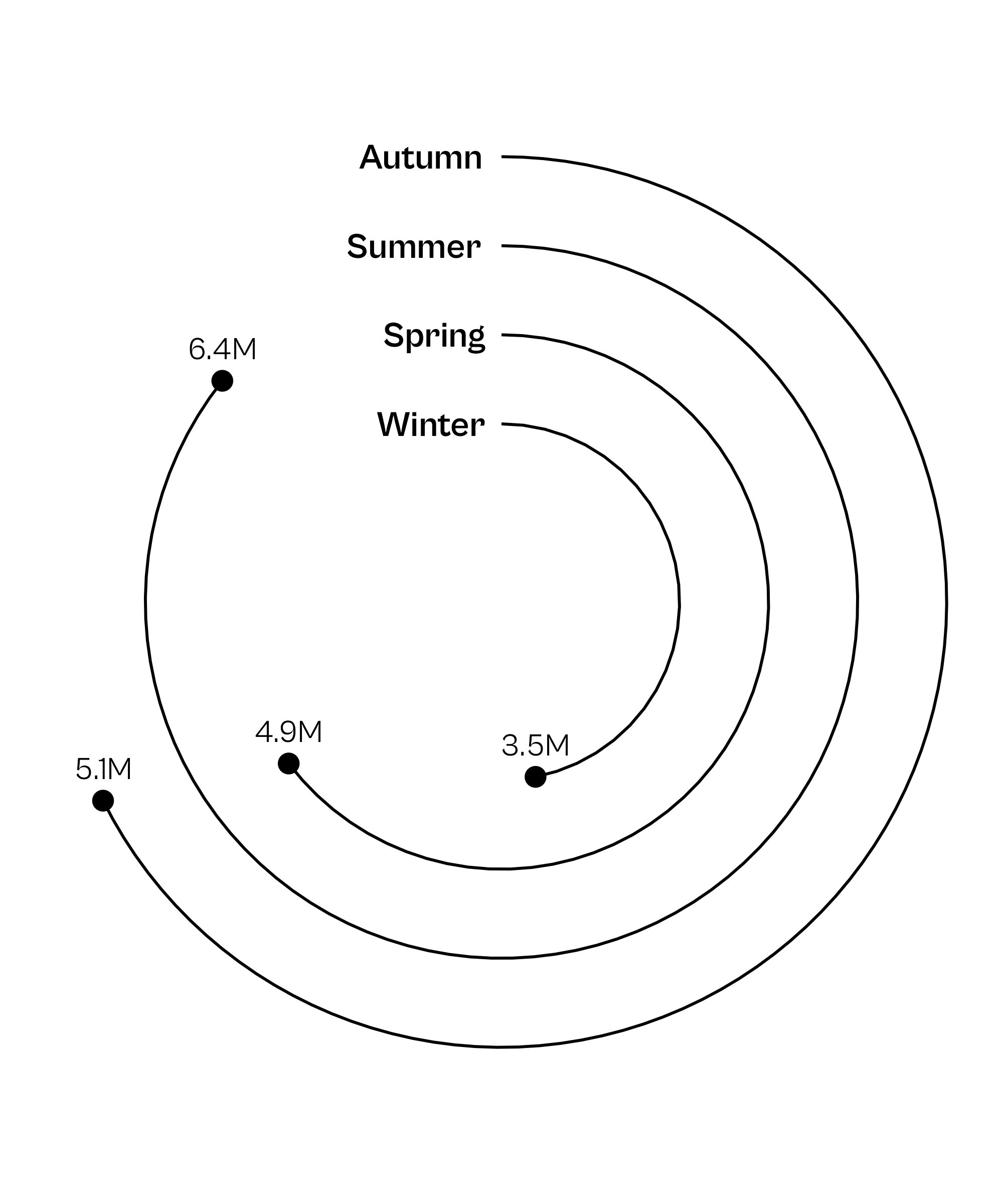

Add a Baseline — ugly but simple

bikes %>%
  group_by(season) %>%
  summarize(count = sum(count)) %>%
  ggplot(aes(x = season, y = count)) +
  geom_point(size = 3) +
  geom_linerange(
    aes(ymin = 0, ymax = count)
  ) +
  geom_hline(yintercept = 0) +
  geom_text(
    aes(label = season, y = 0),
    family = "Cabinet Grotesk", size = 4.5,
    fontface = "bold", hjust = 1.15
  ) +
  coord_polar(theta = "y") +
  scale_x_discrete(
    expand = c(.5, .5)
  ) +
  scale_y_continuous(
    limits = c(0, 7.5*10^6)
  ) +
  theme_void() +
  theme(plot.margin = margin(rep(-100, 4)))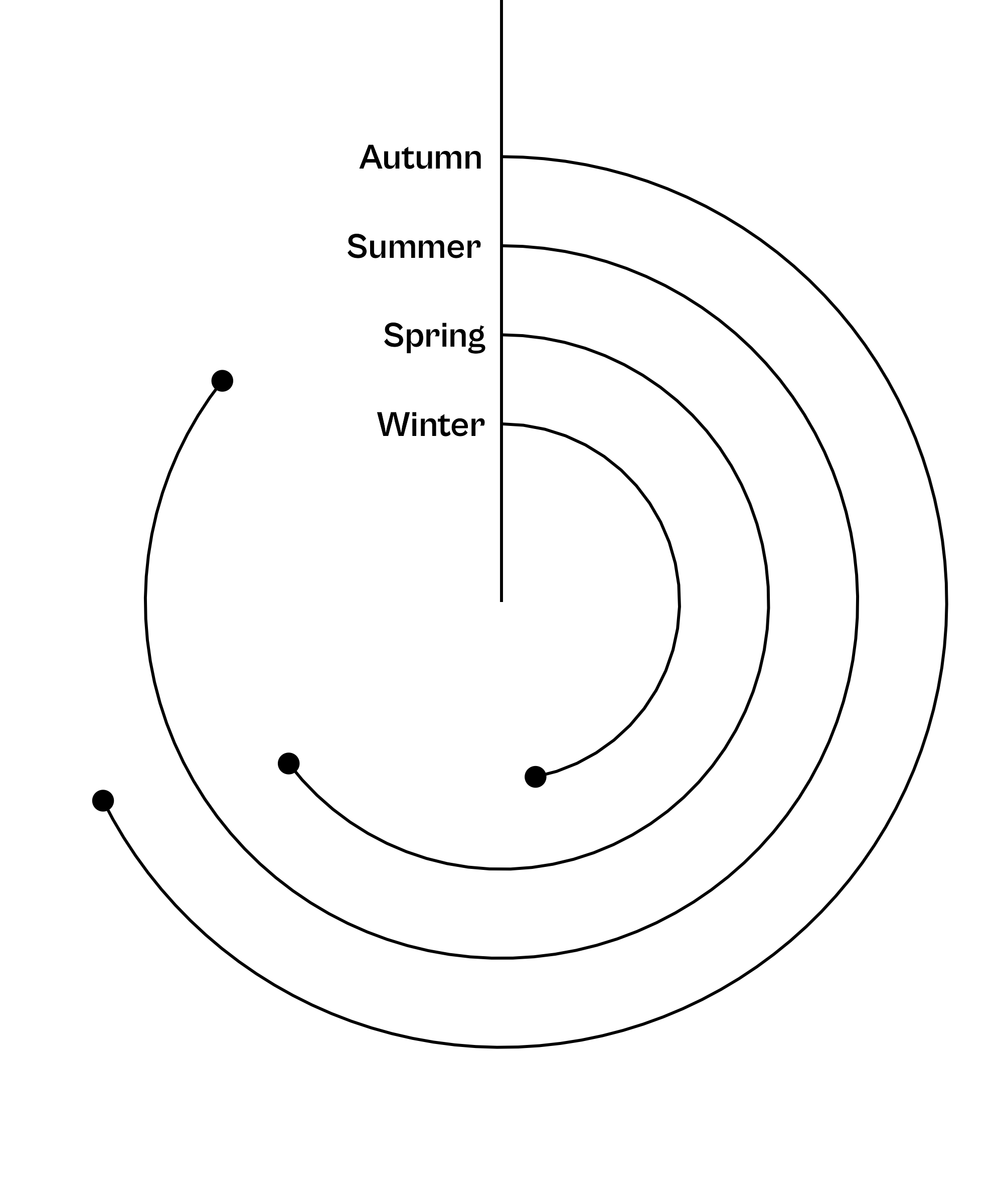

Add a Baseline — nice but unusual

bikes %>%
  group_by(season) %>%
  summarize(count = sum(count)) %>%
  ggplot(aes(x = season, y = count)) +
  geom_point(size = 3) +
  geom_linerange(
    aes(ymin = 0, ymax = count)
  ) +
  geom_linerange(
    xmin = .7, xmax = 4.3, y = 0
  ) +
  geom_text(
    aes(label = season, y = 0),
    family = "Cabinet Grotesk", size = 4.5,
    fontface = "bold", hjust = 1.15
  ) +
  coord_polar(theta = "y") +
  scale_x_discrete(
    expand = c(.5, .5)
  ) +
  scale_y_continuous(
    limits = c(0, 7.5*10^6)
  ) +
  theme_void() +
  theme(plot.margin = margin(rep(-100, 4)))

Add a Baseline — yeah, that’s it!

bikes %>%
  group_by(season) %>%
  summarize(count = sum(count)) %>%
  ggplot(aes(x = season, y = count)) +
  geom_point(size = 3) +
  geom_linerange(
    aes(ymin = 0, ymax = count)
  ) +
  annotate(
    geom = "linerange",
    xmin = .7, xmax = 4.3, y = 0
  )  +
  geom_text(
    aes(label = season, y = 0),
    family = "Cabinet Grotesk", size = 4.5,
    fontface = "bold", hjust = 1.15
  ) +
  coord_polar(theta = "y") +
  scale_x_discrete(
    expand = c(.5, .5)
  ) +
  scale_y_continuous(
    limits = c(0, 7.5*10^6)
  ) +
  theme_void() +
  theme(plot.margin = margin(rep(-100, 4)))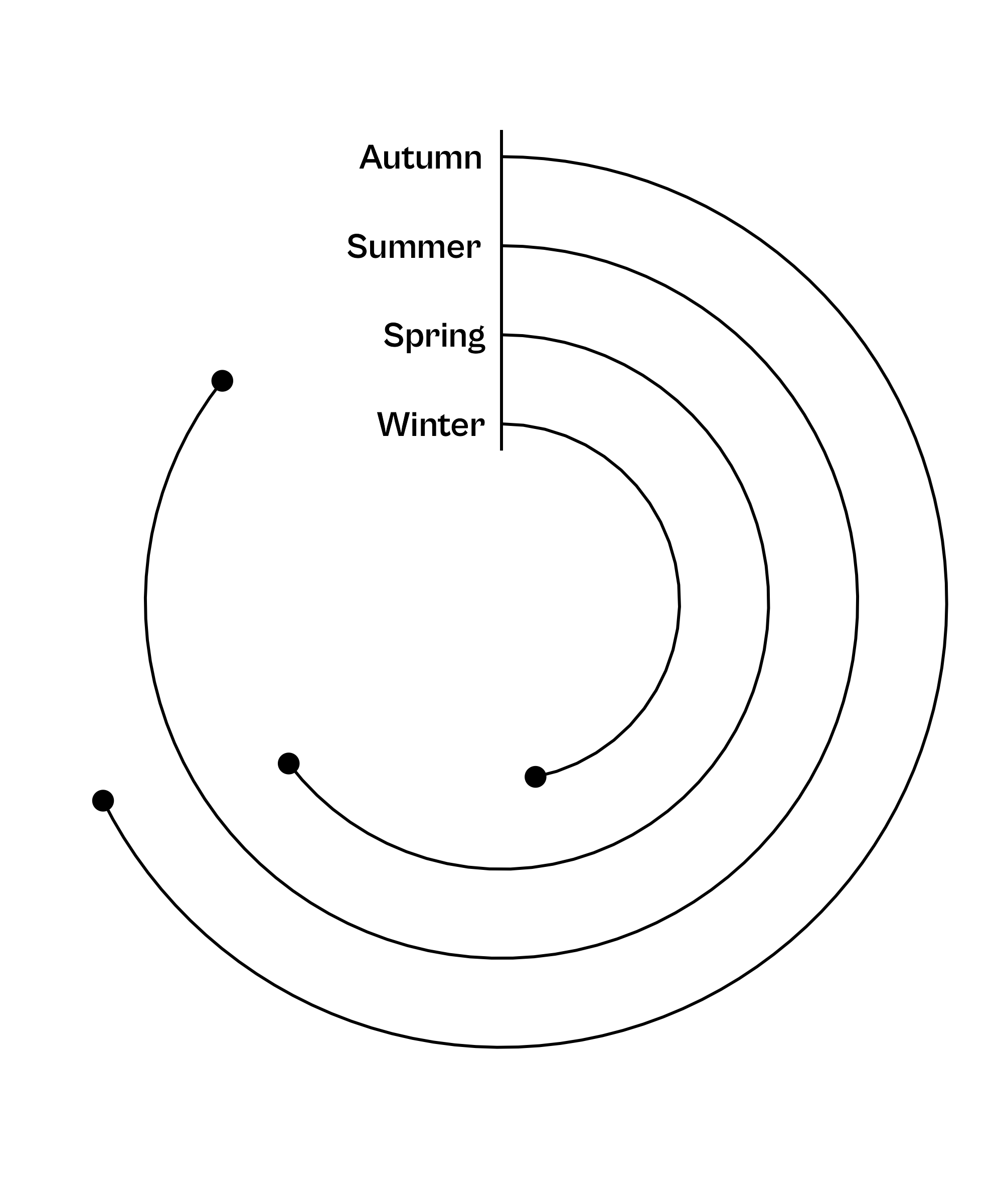

Solution using stat_summary()

ggplot(bikes, aes(x = as.numeric(season), y = count)) +
  stat_summary(
    geom = "point", fun = "sum", size = 3
  ) +
  stat_summary(
    geom = "linerange", ymin = 0,
    fun.max = function(y) sum(y)
  ) +
  stat_summary(
    geom = "text",
    aes(
      label = season,
      y = 0
    ),
    family = "Cabinet Grotesk", size = 4.5,
    fontface = "bold", hjust = 1.15
  ) +
  annotate(
    geom = "linerange",
    xmin = .7, xmax = 4.3, y = 0
  ) +
  coord_polar(theta = "y") +
  scale_x_discrete(
    expand = c(.5, .5)
  ) +
  scale_y_continuous(
    limits = c(0, 7.5*10^6)
  ) +
  theme_void() +
  theme(plot.margin = margin(rep(-100, 4)))