# A tibble: 344 x 8
   species island    bill_length_mm bill_depth_mm flipper_length_mm body_mass_g
   <fct>   <fct>              <dbl>         <dbl>             <int>       <int>
 1 Adelie  Torgersen           39.1          18.7               181        3750
 2 Adelie  Torgersen           39.5          17.4               186        3800
 3 Adelie  Torgersen           40.3          18                 195        3250
 4 Adelie  Torgersen           NA            NA                  NA          NA
 5 Adelie  Torgersen           36.7          19.3               193        3450
 6 Adelie  Torgersen           39.3          20.6               190        3650
 7 Adelie  Torgersen           38.9          17.8               181        3625
 8 Adelie  Torgersen           39.2          19.6               195        4675
 9 Adelie  Torgersen           34.1          18.1               193        3475
10 Adelie  Torgersen           42            20.2               190        4250
# ... with 334 more rows, and 2 more variables: sex <fct>, year <int>Graphic Design with ggplot2
Working with Labels and Annotations:
Solution Exercise 1
Cédric Scherer // rstudio::conf // July 2022
Exercise 1
- {ggtext} also comes with some new geom’s. Explore those and other options on the package webpage: wilkelab.rg/ggtext.
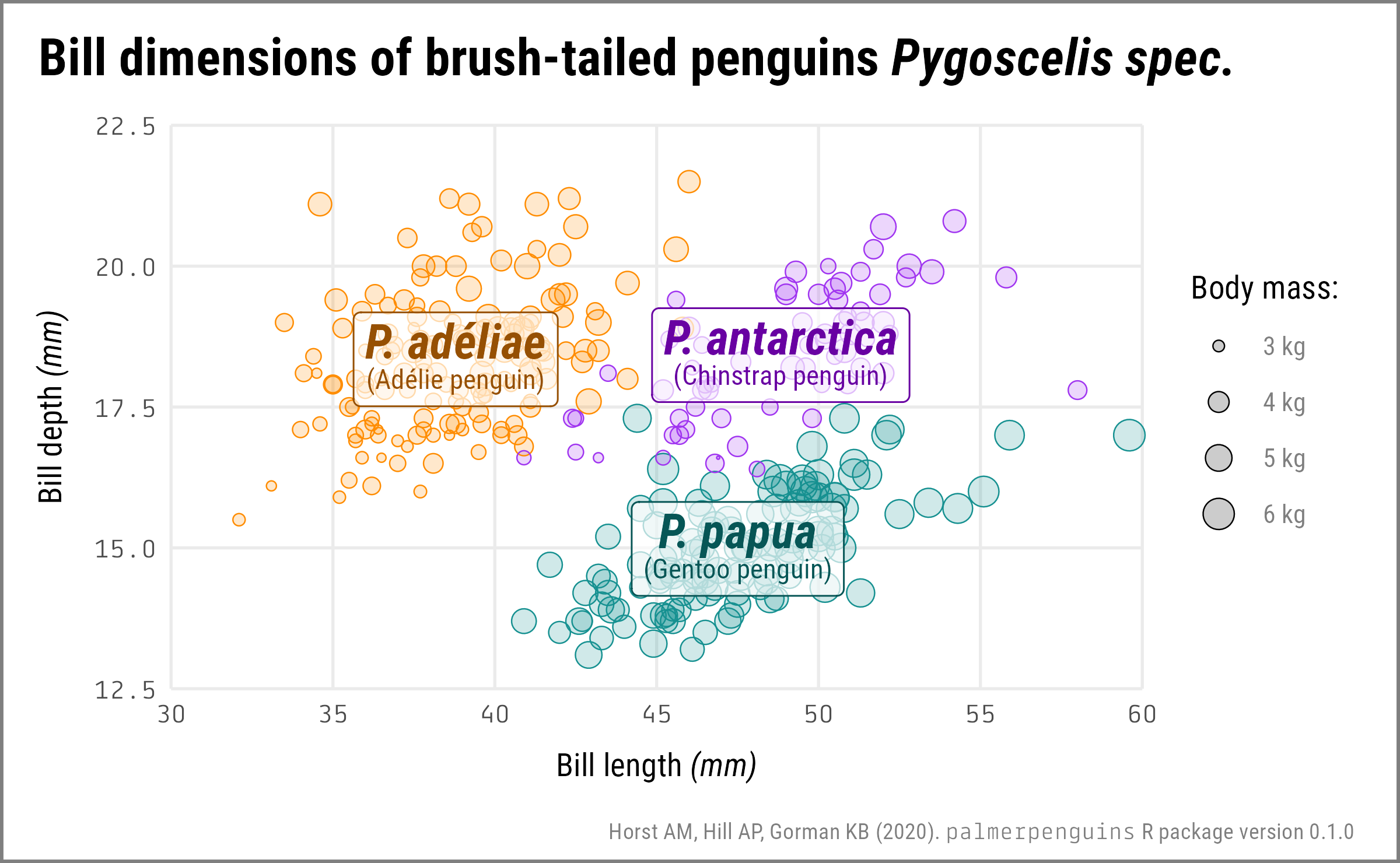
- Create the following visualization, as close as possible, with the
penguinsdataset which is provided by the {palmerpenguins} package.- For the species labels, you likely have to create a summary data set.
- Use the {ggtext} geometries and theme elements to format the labels.
- Also, make use of the other components such as scales, original theme, and theme customization.
The Data Set
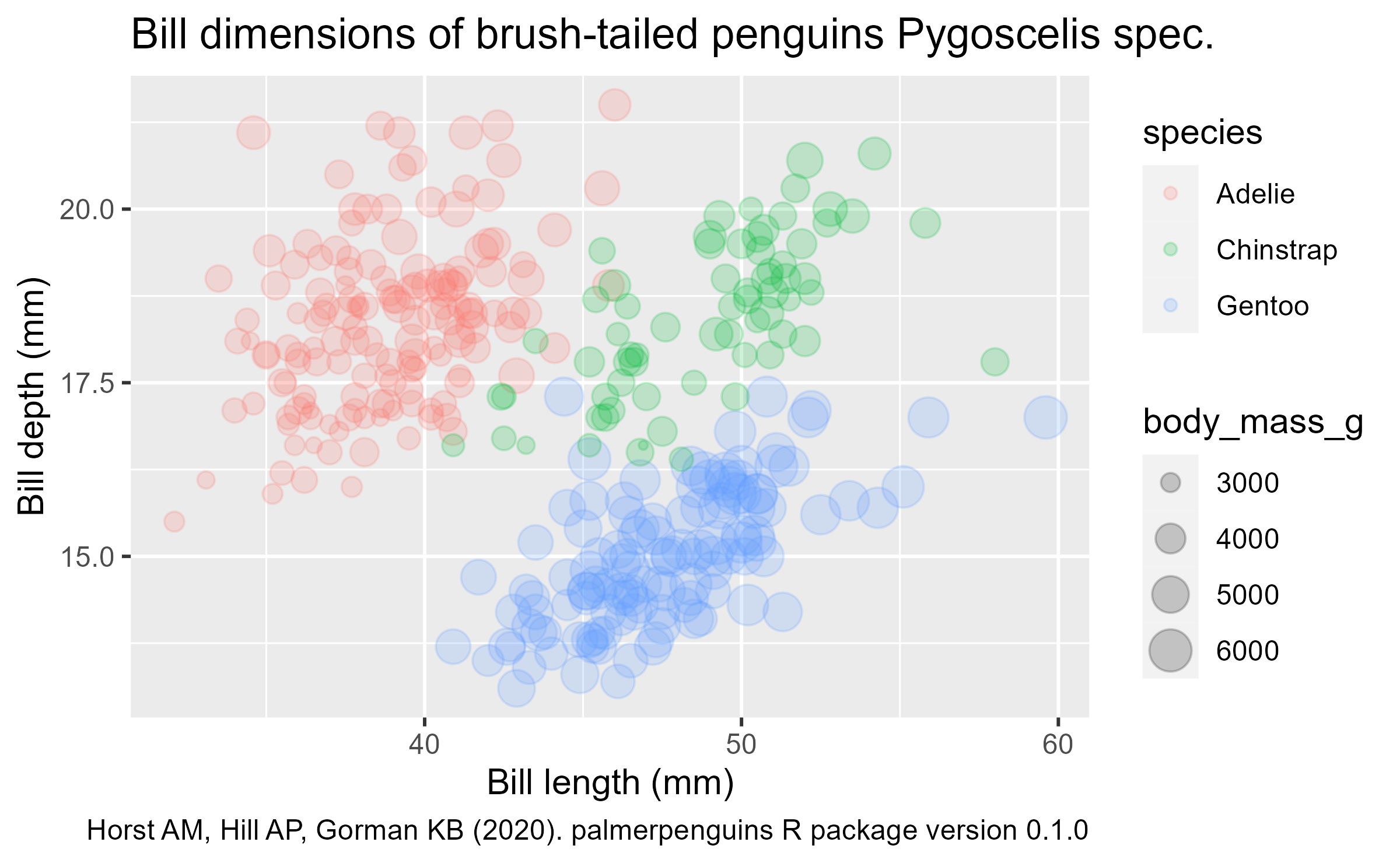
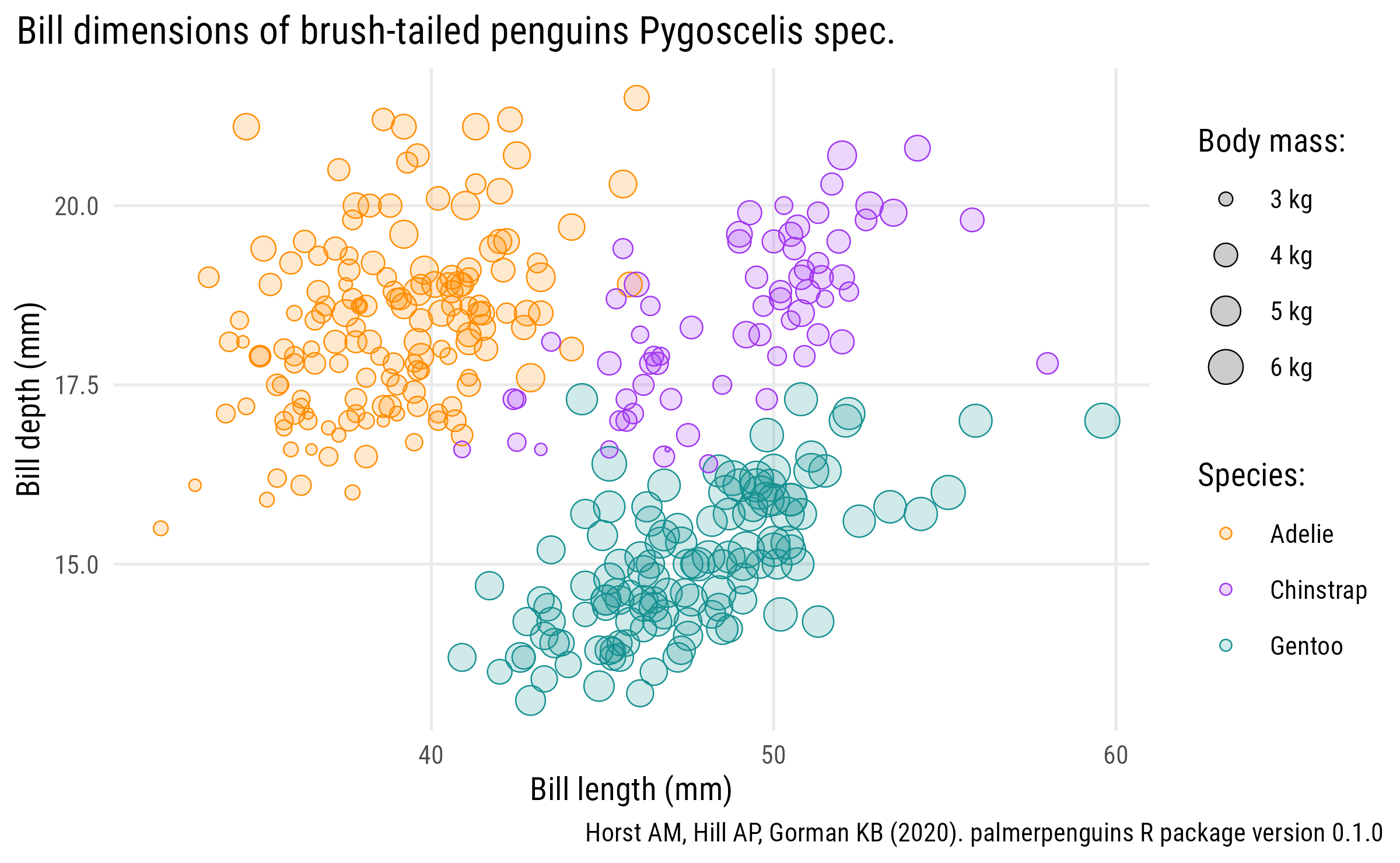
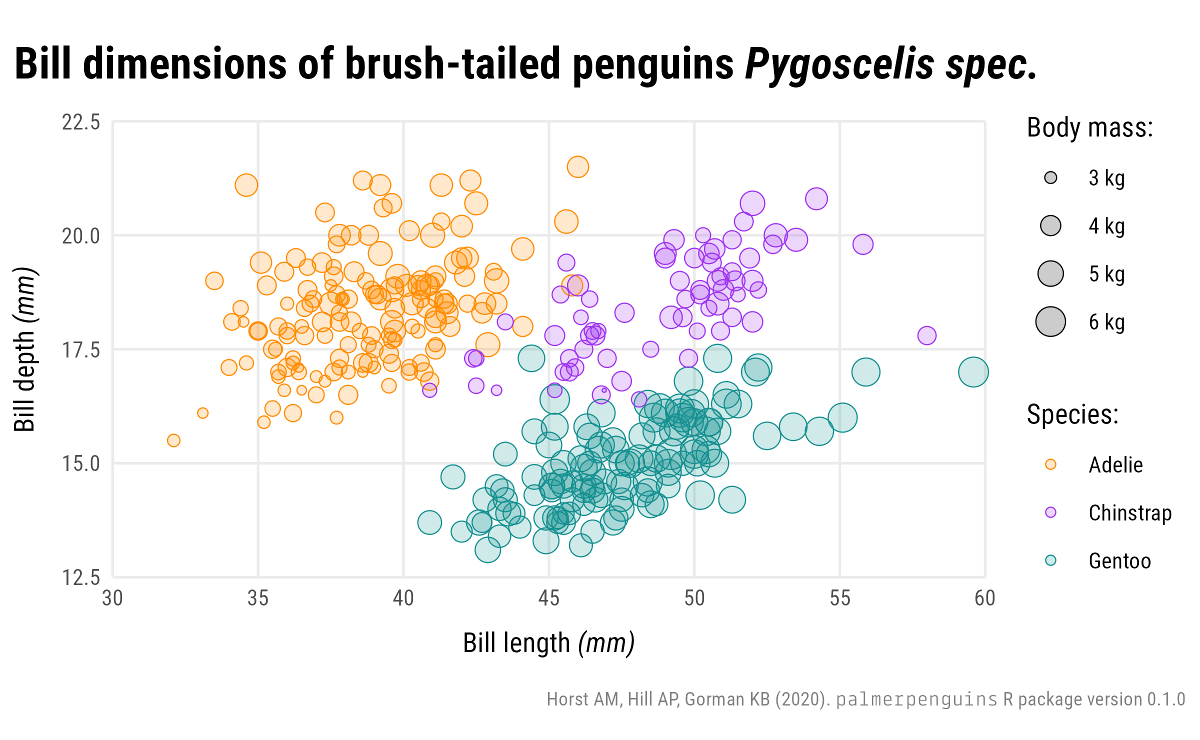
Create a Labeled Bubble Chart
ggplot(
    penguins,
    aes(x = bill_length_mm, y = bill_depth_mm,
        color = species, size = body_mass_g)
  ) +
  geom_point(alpha = .2) +
  labs(
    x = "Bill length (mm)",
    y = "Bill depth (mm)",
    title = "Bill dimensions of brush-tailed penguins Pygoscelis spec.",
    caption = "Horst AM, Hill AP, Gorman KB (2020). palmerpenguins R package version 0.1.0"
  )
A Labelled Bubble Plot
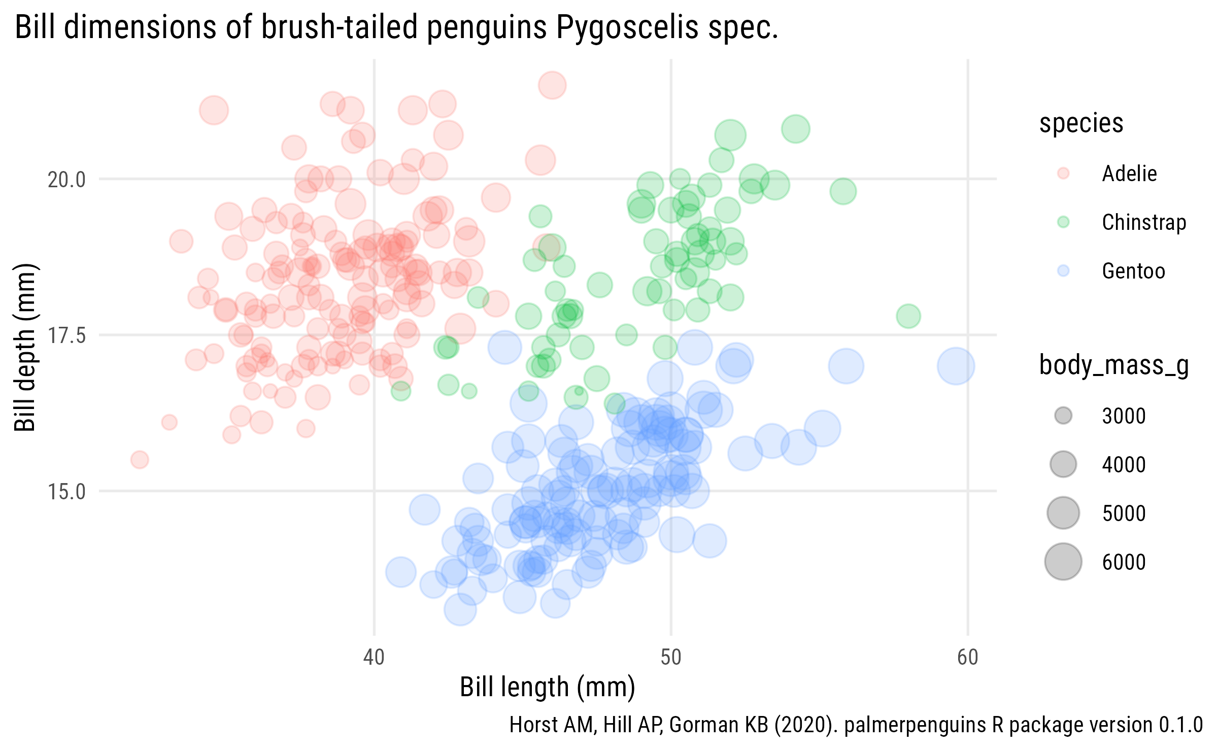
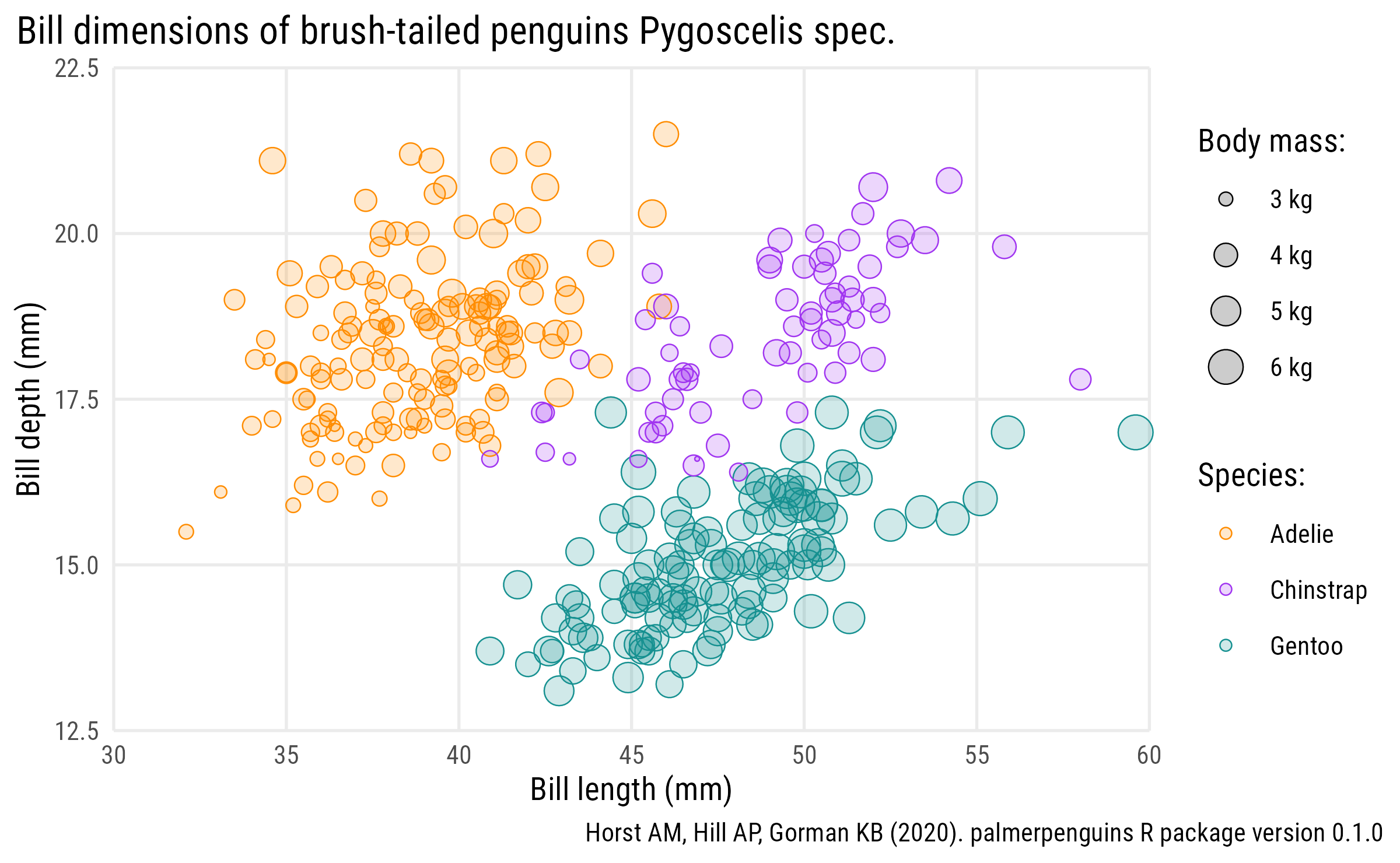
Add a Custom Theme
ggplot(
    penguins,
    aes(x = bill_length_mm, y = bill_depth_mm,
        color = species, size = body_mass_g)
  ) +
  geom_point(alpha = .2) +
  labs(
    x = "Bill length (mm)",
    y = "Bill depth (mm)",
    title = "Bill dimensions of brush-tailed penguins Pygoscelis spec.",
    caption = "Horst AM, Hill AP, Gorman KB (2020). palmerpenguins R package version 0.1.0"
  ) +
  theme_minimal(base_size = 10, base_family = "Roboto Condensed") +
  theme(
    plot.title.position = "plot",
    plot.caption.position = "plot",
    panel.grid.minor = element_blank()
  )
Add a Custom Theme
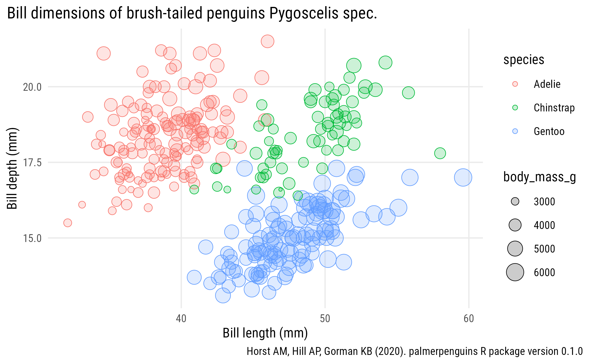
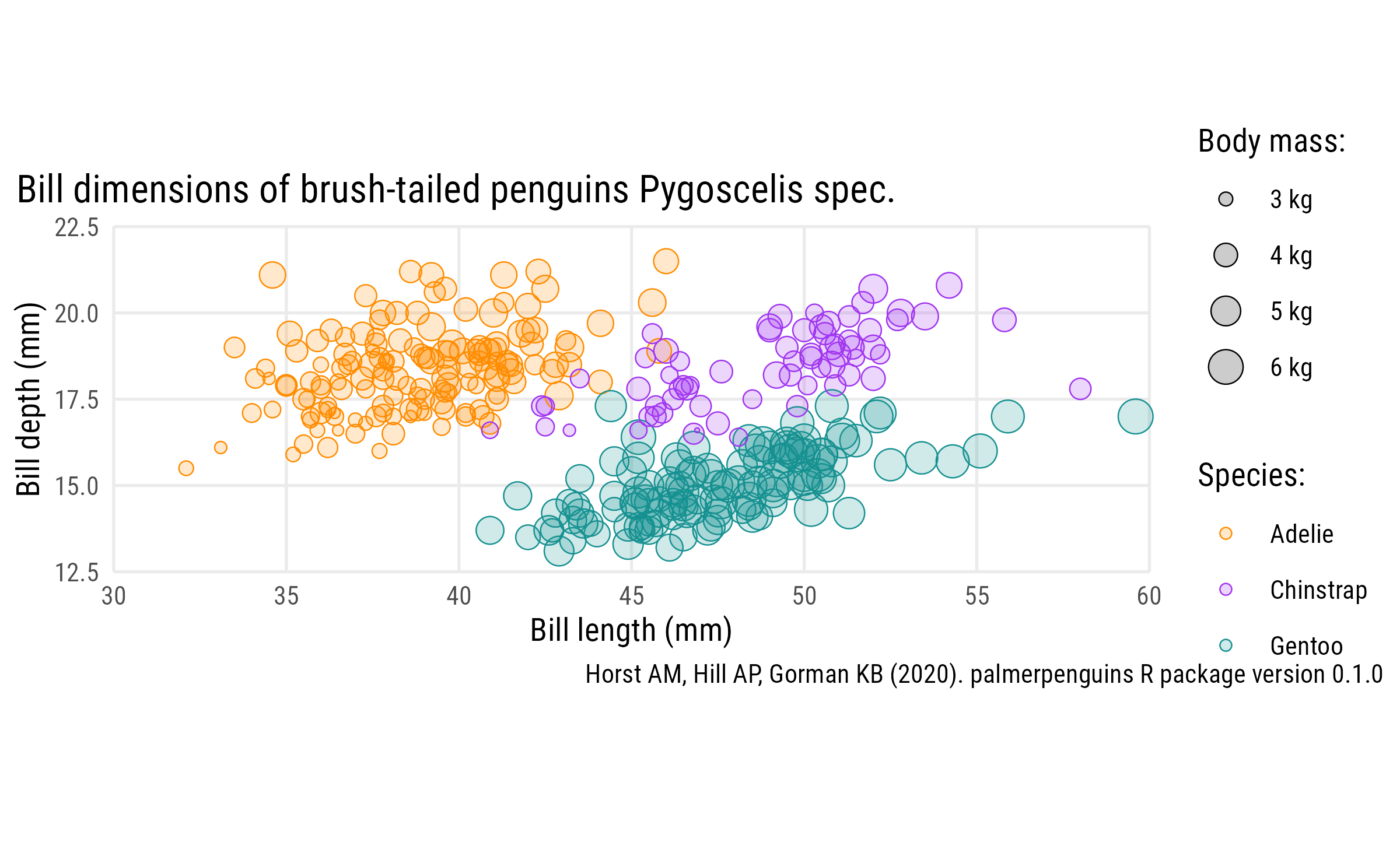
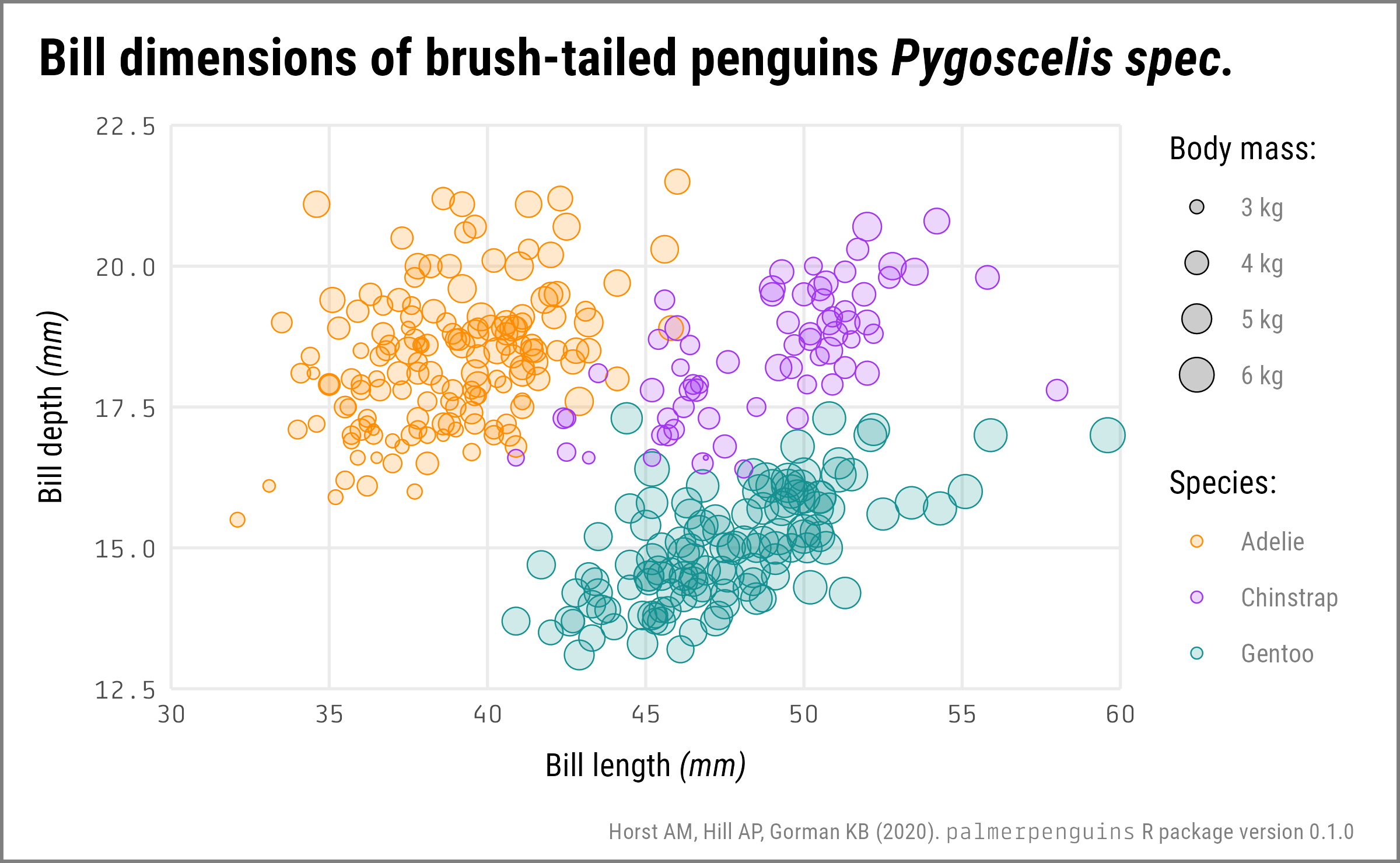
Add an Outline
p1 <-
  ggplot(
    penguins,
    aes(x = bill_length_mm, y = bill_depth_mm,
        color = species, size = body_mass_g)
  ) +
  geom_point(alpha = .2, stroke = .3) +
  geom_point(shape = 1, stroke = .3) +
  labs(
    x = "Bill length (mm)",
    y = "Bill depth (mm)",
    title = "Bill dimensions of brush-tailed penguins Pygoscelis spec.",
    caption = "Horst AM, Hill AP, Gorman KB (2020). palmerpenguins R package version 0.1.0"
  ) +
  theme_minimal(base_size = 10, base_family = "Roboto Condensed") +
  theme(
    plot.title.position = "plot",
    plot.caption.position = "plot",
    panel.grid.minor = element_blank()
  )

p1
Add an Outline
Style Color Legend
Style Color Legend

Style Size Legend
Style Size Legend
Adjust Axes
Adjust Axes

Adjust Axes
Adjust Axes
Fixed Coordinate System?
Fixed Coordinate System?
Format Labels with {ggtext}
Format Labels with {ggtext}
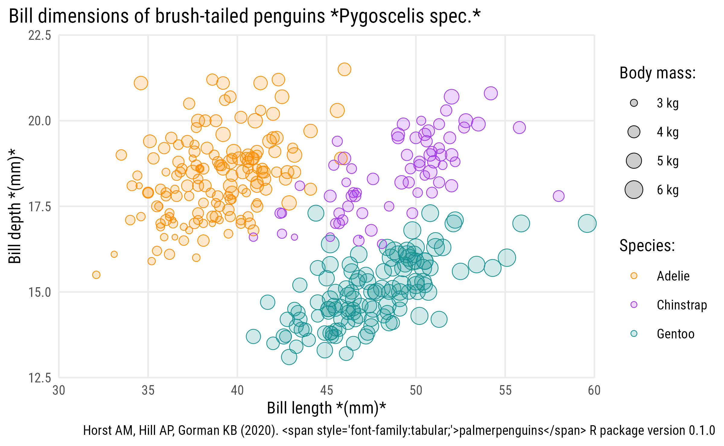
Format Labels with {ggtext}
library(ggtext)

p4 <- p3 +
  labs(
    x = "Bill length *(mm)*",
    y = "Bill depth *(mm)*",
    title = "Bill dimensions of brush-tailed penguins *Pygoscelis spec.*",
    caption = "Horst AM, Hill AP, Gorman KB (2020). <span style='font-family:tabular;'>palmerpenguins</span> R package version 0.1.0"
  ) +
  theme(
    plot.title = element_markdown(
      face = "bold", size = 16, margin = margin(12, 0, 12, 0)
    ),
    plot.caption = element_markdown(
      size = 7, color = "grey50", margin = margin(12, 0, 6, 0)
    ),
    axis.title.x = element_markdown(margin = margin(t = 8)),
    axis.title.y = element_markdown(margin = margin(r = 8))
  )

p4
Format Labels with {ggtext}
Style Other Theme Elements
Style Other Theme Elements
Create the Summary Data
library(tidyverse)

penguins_labs <-
  penguins %>%
  group_by(species) %>%
  summarize(across(starts_with("bill"), ~ mean(.x, na.rm = TRUE))) %>%
  mutate(
    species_lab = case_when(
      species == "Adelie" ~ "<b style='font-size:15pt;'>*P. adéliae*</b><br>(Adélie penguin)",
      species == "Chinstrap" ~ "<b style='font-size:15pt;'>*P. antarctica*</b><br>(Chinstrap penguin)",
      species == "Gentoo" ~ "<b style='font-size:15pt;'>*P. papua*</b><br>(Gentoo penguin)"
    )
  )

penguins_labs
# A tibble: 3 x 4
species bill_length_mm bill_depth_mm species_lab
<fct> <dbl> <dbl> <chr>
1 Adelie 38.8 18.3 <b style='font-size:15pt;'>*P. adéliae~
2 Chinstrap 48.8 18.4 <b style='font-size:15pt;'>*P. antarct~
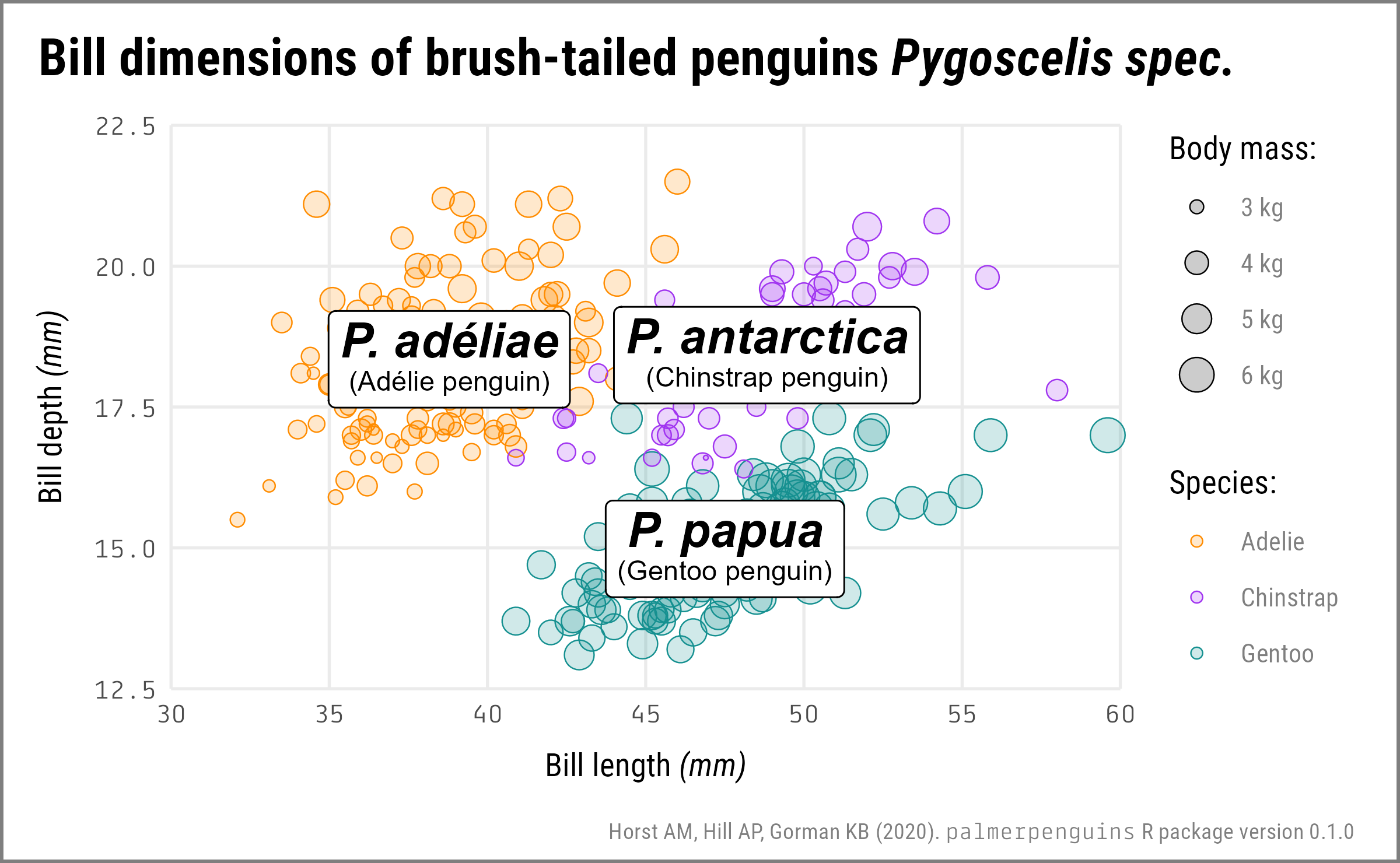
3 Gentoo 47.5 15.0 <b style='font-size:15pt;'>*P. papua*<~Add Species Annotations
Add Species Annotations
Style Species Annotations
Style Species Annotations
Style Species Annotations
Style Species Annotations
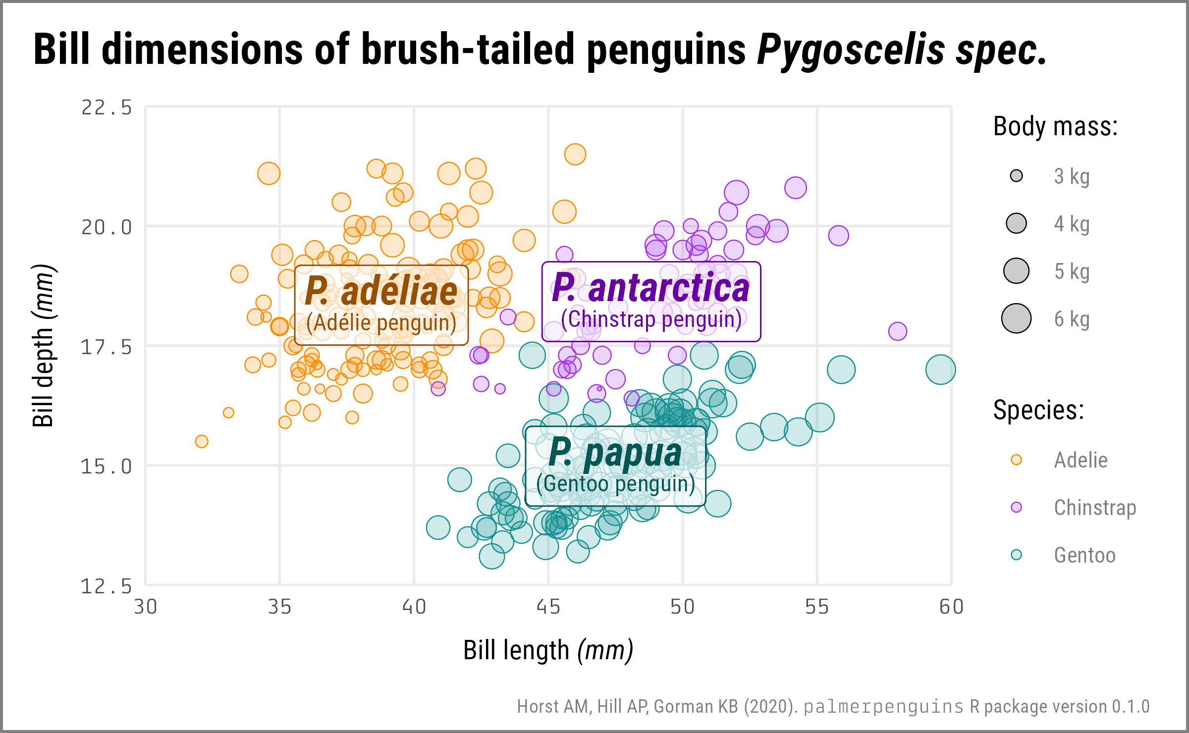
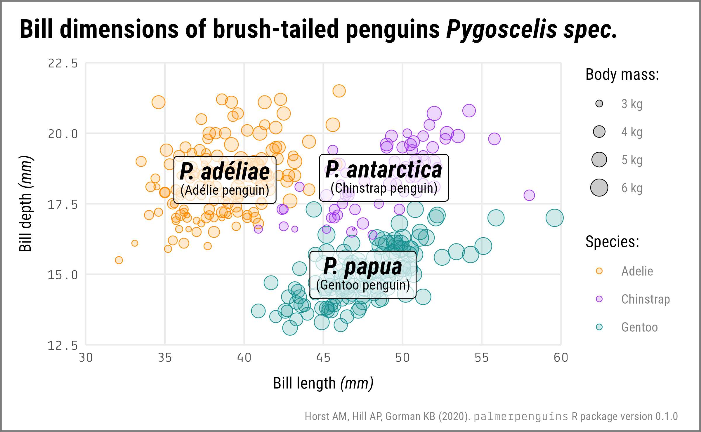
… and Remove Color Legend
p5 +
  geom_richtext(
    data = penguins_labs,
    aes(label = species_lab,
        color = species,
        color = after_scale(colorspace::darken(color, .4))),
    family = "Roboto Condensed",
    size = 3, lineheight = .8,
    fill = "#ffffffab", ## hex-alpha code
    show.legend = FALSE
  ) +
  scale_color_manual(
    guide = "none",
    values = c("#FF8C00", "#A034F0", "#159090")
  )
… and Remove Color Legend
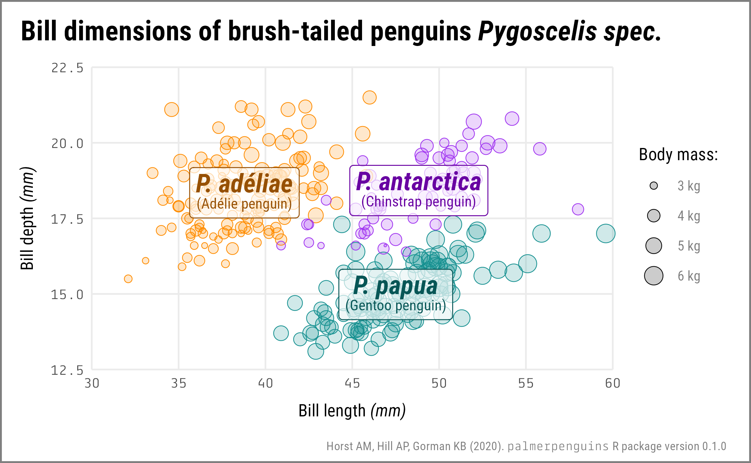
Full Code
library(tidyverse)
library(palmerpenguins)
library(ggtext)

penguins_labs <-
  penguins %>%
  group_by(species) %>%
  summarize(across(starts_with("bill"), ~ mean(.x, na.rm = TRUE))) %>%
  mutate(
    species_lab = case_when(
      species == "Adelie" ~ "<b style='font-size:15pt;'>*P. adéliae*</b><br>(Adélie penguin)",
      species == "Chinstrap" ~ "<b style='font-size:15pt;'>*P. antarctica*</b><br>(Chinstrap penguin)",
      species == "Gentoo" ~ "<b style='font-size:15pt;'>*P. papua*</b><br>(Gentoo penguin)"
    )
  )

ggplot(
    penguins,
    aes(x = bill_length_mm, y = bill_depth_mm,
        color = species, size = body_mass_g)
  ) +
  geom_point(alpha = .2, stroke = .3) +
  geom_point(shape = 1, stroke = .3) +
  geom_richtext(
    data = penguins_labs,
    aes(label = species_lab,
        color = species,
        color = after_scale(colorspace::darken(color, .4))),
    family = "Roboto Condensed",
    size = 3, lineheight = .8,
    fill = "#ffffffab", ## hex-alpha code
    show.legend = FALSE
  ) +
  coord_cartesian(
    expand = FALSE,
    clip = "off"
  )  +
  scale_x_continuous(
    limits = c(30, 60),
    breaks = 6:12*5
  ) +
  scale_y_continuous(
    limits = c(12.5, 22.5),
    breaks = seq(12.5, 22.5, by = 2.5)
  ) +
  scale_color_manual(
    guide = "none",
    values = c("#FF8C00", "#A034F0", "#159090")
  ) +
  scale_size(
    name = "Body mass:",
    breaks = 3:6 * 1000,
    labels = function(x) paste(x / 1000, "kg"),
    range = c(.25, 4.5)
  ) +
  labs(
    x = "Bill length *(mm)*",
    y = "Bill depth *(mm)*",
    title = "Bill dimensions of brush-tailed penguins *Pygoscelis spec.*",
    caption = "Horst AM, Hill AP, Gorman KB (2020). <span style='font-family:tabular;'>palmerpenguins</span> R package version 0.1.0"
  ) +
  theme_minimal(
    base_size = 10, base_family = "Roboto Condensed"
  ) +
  theme(
    plot.title = element_markdown(
      face = "bold", size = 16, margin = margin(12, 0, 12, 0)
    ),
    plot.title.position = "plot",
    plot.caption = element_markdown(
      size = 7, color = "grey50",
      margin = margin(12, 0, 6, 0)
    ),
    plot.caption.position = "plot",
    axis.text = element_text(family = "Tabular"),
    axis.title.x = element_markdown(margin = margin(t = 8)),
    axis.title.y = element_markdown(margin = margin(r = 8)),
    panel.grid.minor = element_blank(),
    legend.text = element_text(color = "grey50"),
    plot.margin = margin(0, 14, 0, 12),
    plot.background = element_rect(fill = NA, color = "grey50", size = 1)
  )
Cédric Scherer // rstudio::conf // July 2022