Graphic Design with ggplot2
Working with Colors:
Solution Exercise 1
Cédric Scherer // rstudio::conf // July 2022
Exercise
- Create a similar visualization as close as possible:

Import the Data Set
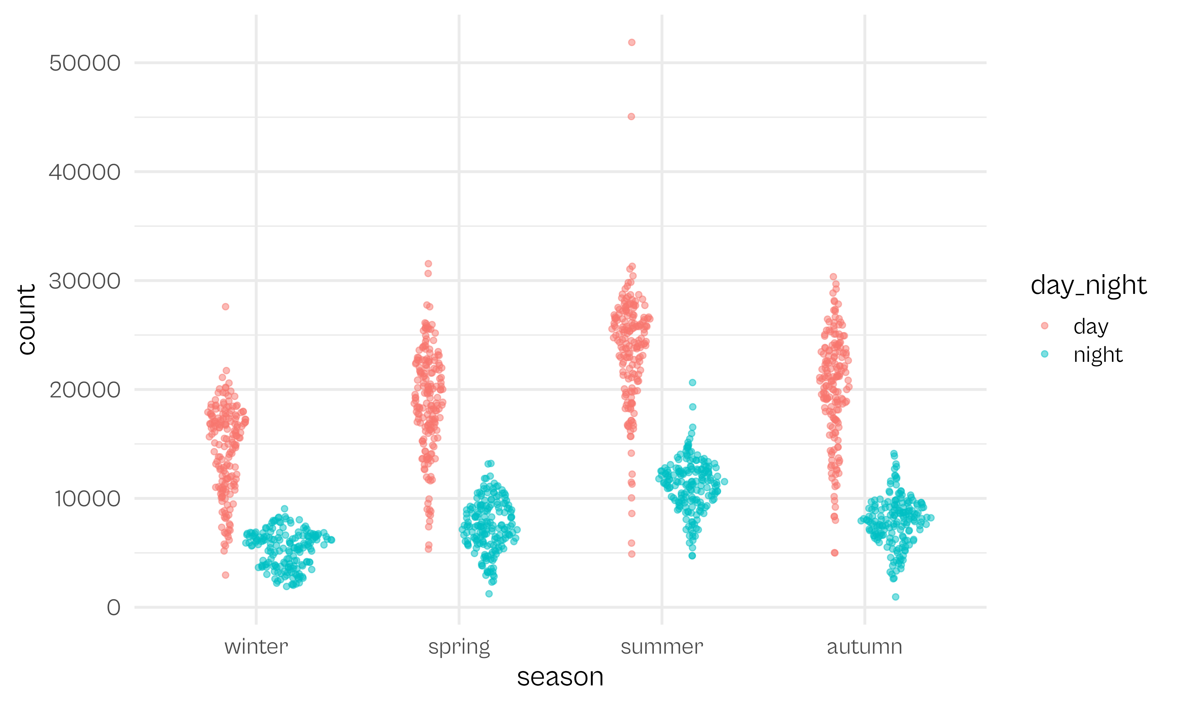
Create Sina Plot
Create Sina Plot
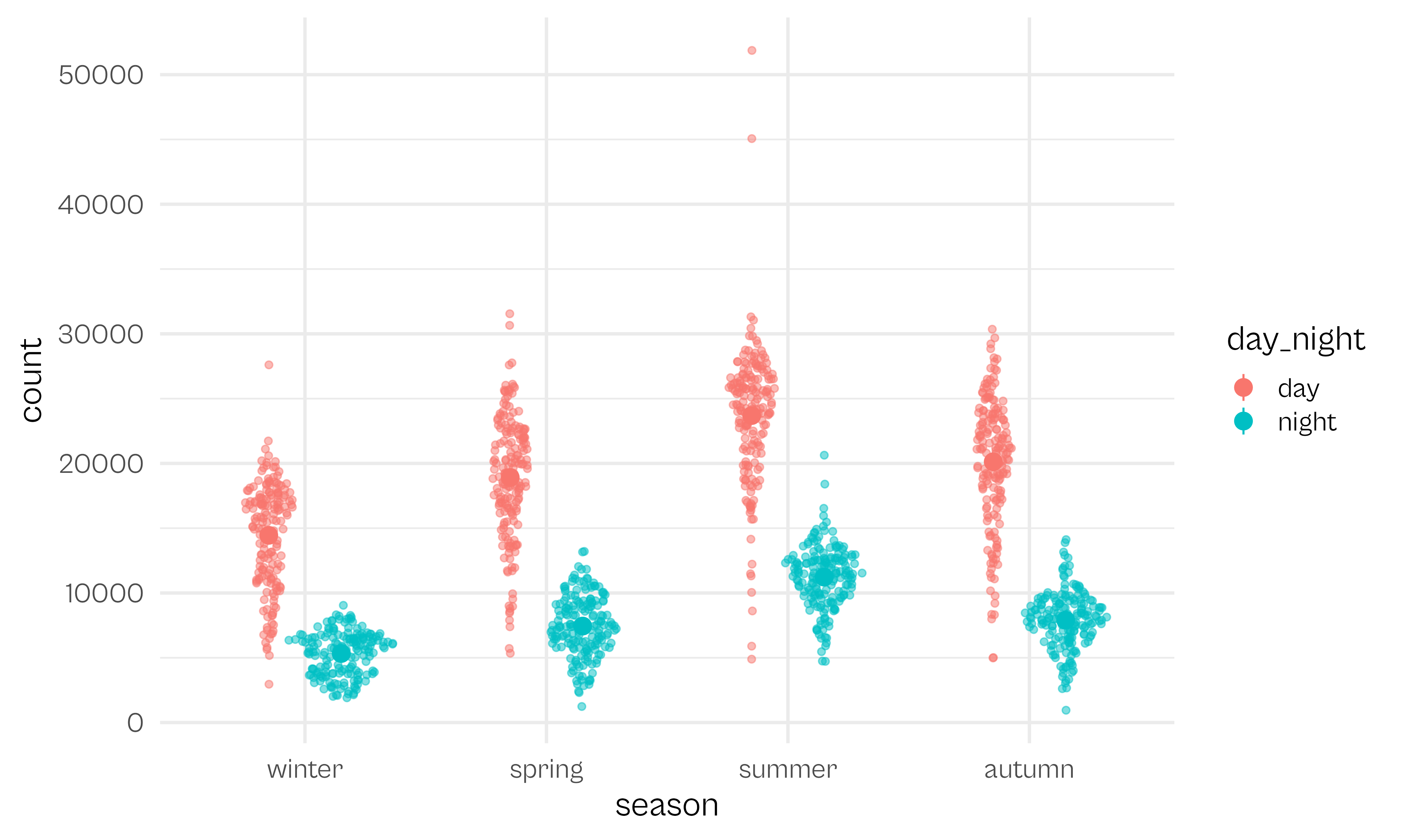
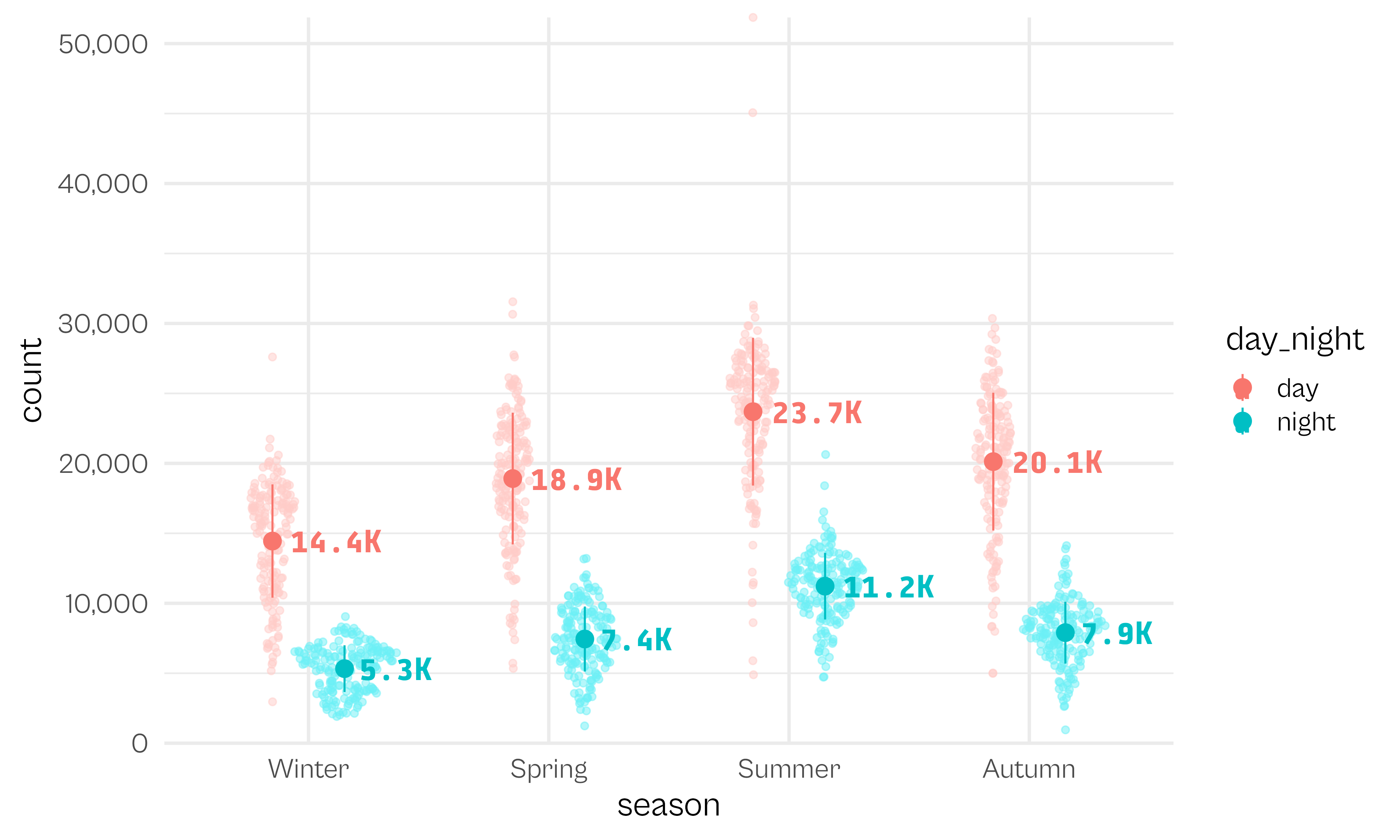
Add Errorbars
Add Errorbars
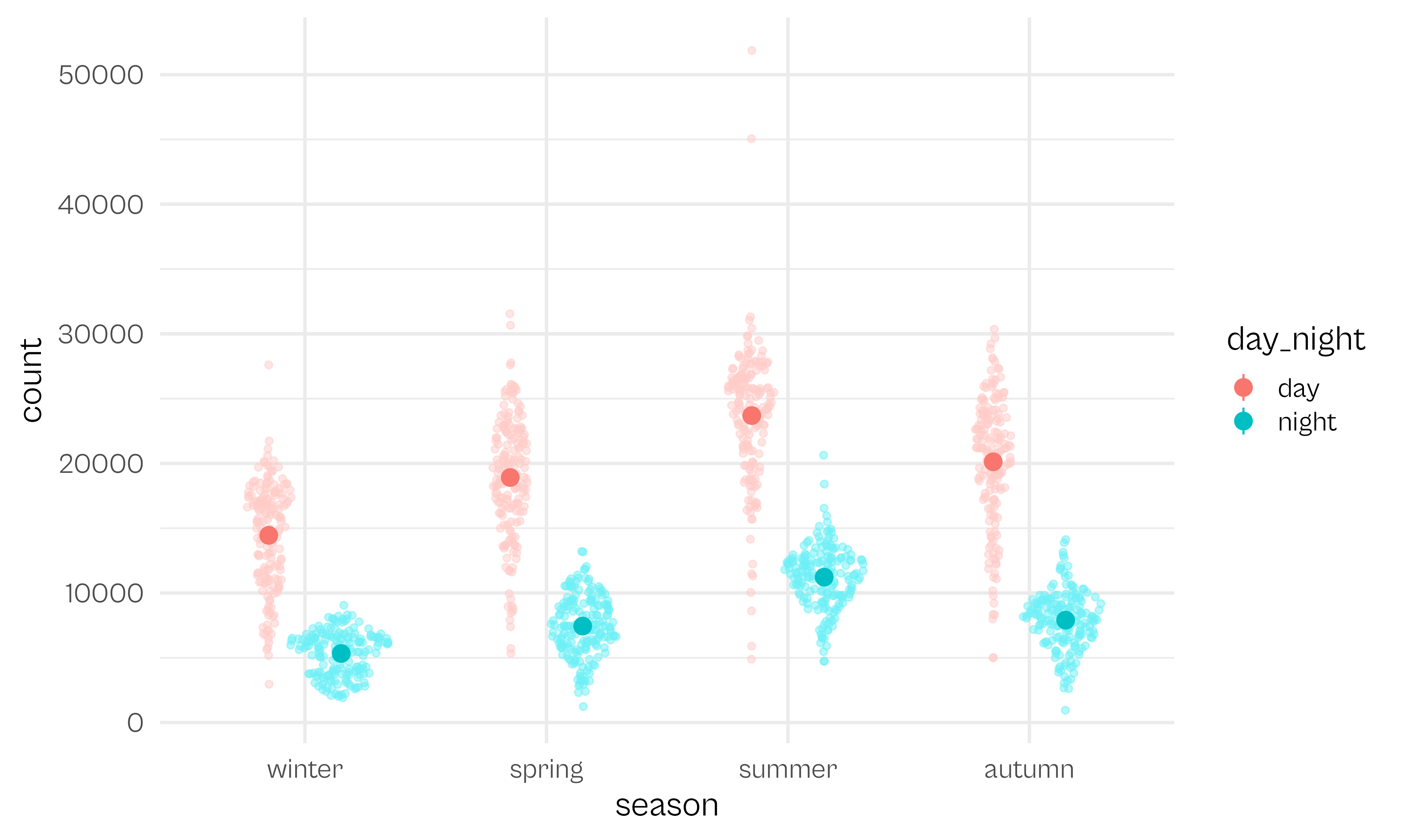
Use Lighter Point Colors
ggplot(
    bikes,
    aes(x = season, y = count)
  ) +
  ggforce::geom_sina(
    aes(color = stage(
      day_night,
      after_scale = lighten(color, .6)
    )),
    position = position_dodge(width = .6),
    alpha = .5
  ) +
  stat_summary(
    aes(color = day_night),
    position = position_dodge(width = .6),
    size = .8
  ) +
  theme_minimal(
    base_size = 18,
    base_family = "Cabinet Grotesk"
  )
Use Lighter Point Colors
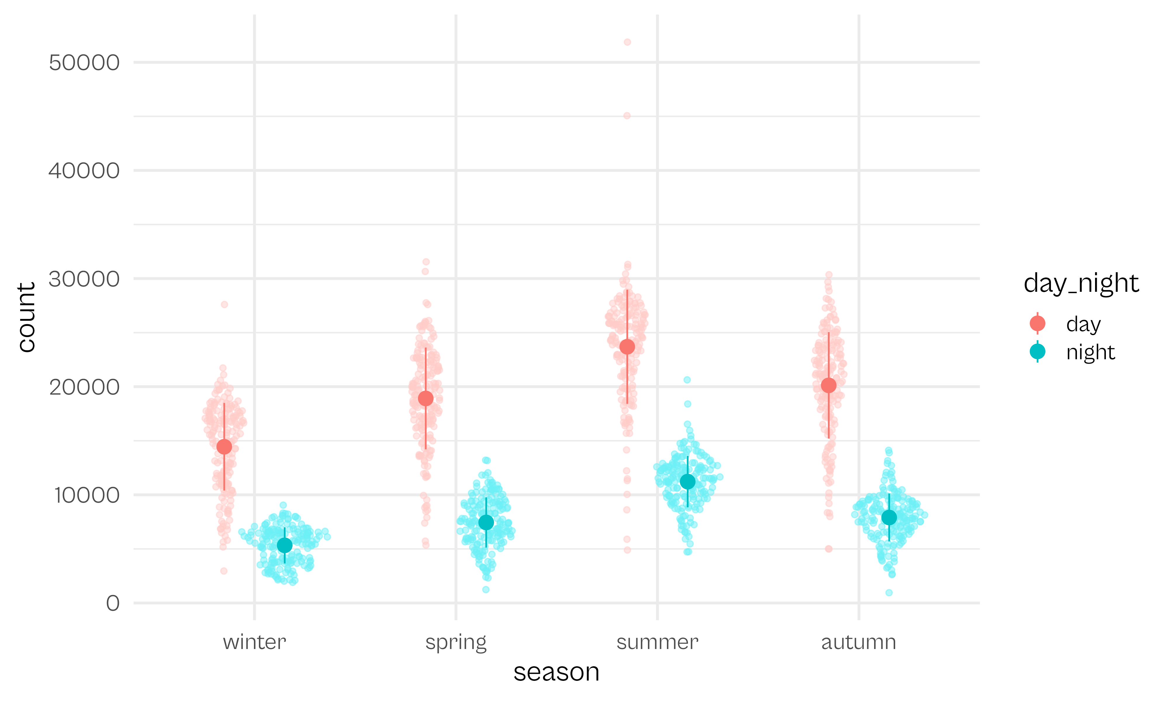
Use Standard Deviation
p1 <- ggplot(
    bikes,
    aes(x = season, y = count)
  ) +
  ggforce::geom_sina(
    aes(color = stage(
      day_night,
      after_scale = lighten(color, .6)
    )),
    position = position_dodge(width = .6),
    alpha = .5
  ) +
  stat_summary(
    aes(color = day_night),
    fun = mean,
    fun.max = function(y) mean(y) + sd(y),
    fun.min = function(y) mean(y) - sd(y),
    position = position_dodge(width = .6),
    size = .8
  ) +
  theme_minimal(
    base_size = 18,
    base_family = "Cabinet Grotesk"
  )

p1
Add Annotations
Add Annotations
Add Annotations

Adjust Axes + Clipping
Adjust Axes + Clipping
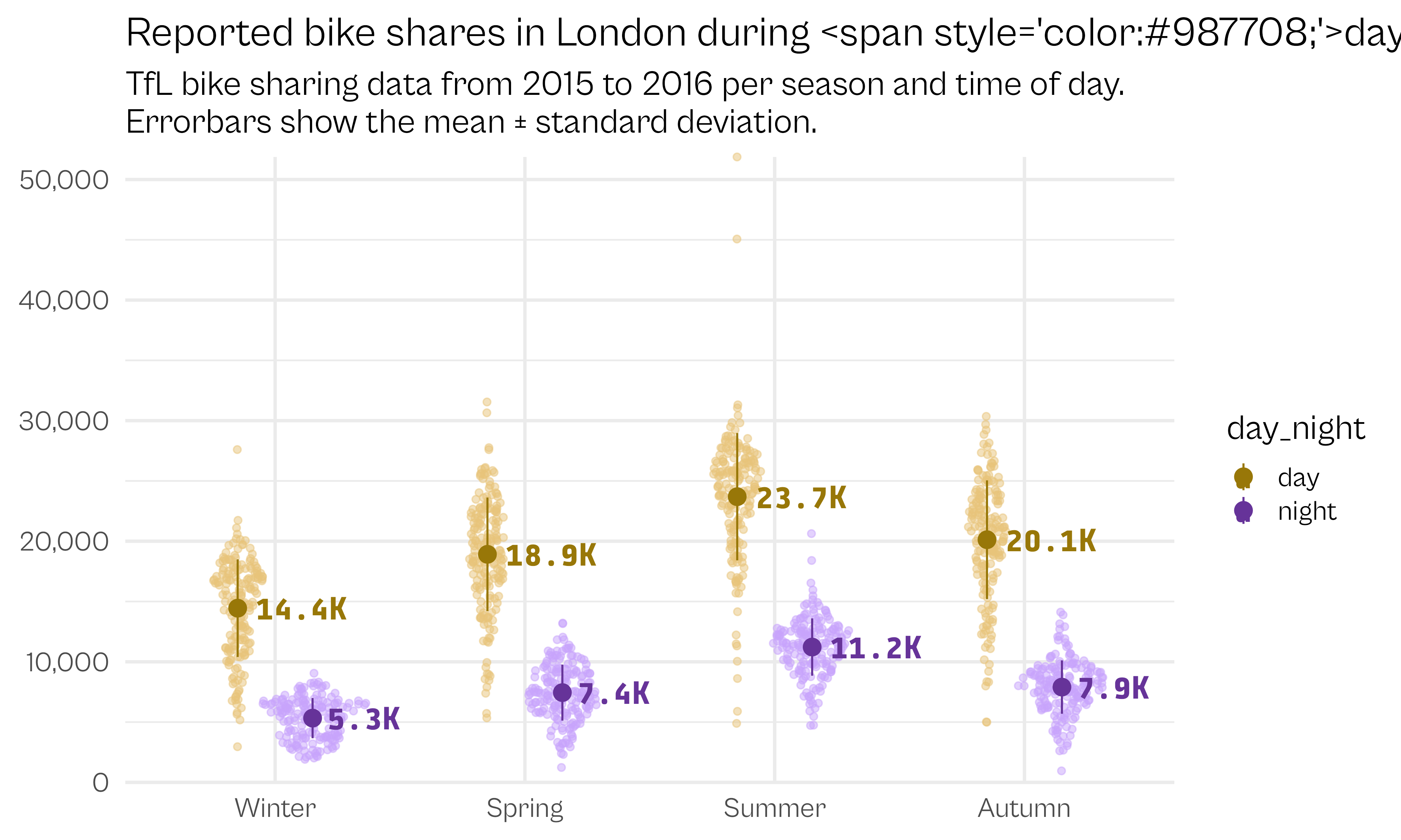
Add Colors + Labels
colors <- c("#987708", "#663399")

p4 <- p3  +
  scale_color_manual(
    values = colors
  ) +
  labs(
    x = NULL, y = NULL,
    title = paste0("Reported bike shares in London during <span style='color:", colors[1], ";'>day</span> and <span style='color:", colors[2], ";'>night</span> times"),
    subtitle = "TfL bike sharing data from 2015 to 2016 per season and time of day.\nErrorbars show the mean ± standard deviation."
  )

p4
Add Colors + Labels
Theme Styling
p4 +
  theme(
    legend.position = "none",
    panel.grid.major.x = element_blank(),
    panel.grid.minor = element_blank(),
    plot.title.position = "plot",
    plot.title = ggtext::element_markdown(face = "bold", size = 26),
    plot.subtitle = element_text(color = "grey30", margin = margin(t = 6, b = 12)),
    axis.text.x = element_text(size = 17, face = "bold"),
    axis.text.y = element_text(family = "Tabular"),
    axis.line.x = element_line(size = 1.2, color = "grey65"),
    plot.margin = margin(rep(15, 4))
  )
Theme Styling
Full Code
library(tidyverse)
library(colorspace)
library(ggtext)

bikes <- readr::read_csv(
  "https://raw.githubusercontent.com/z3tt/graphic-design-ggplot2/main/data/london-bikes-custom.csv",
  col_types = "Dcfffilllddddc"
)

bikes$season <- forcats::fct_inorder(bikes$season)

colors <- c("#987708", "#663399")

ggplot(bikes, aes(x = season, y = count)) +
  ggforce::geom_sina(
    aes(
      color = stage(
        day_night, after_scale = lighten(color, .6)
    )),
    position = position_dodge(width = .6),
    alpha = .5
  ) +
  stat_summary(
    aes(color = day_night),
    position = position_dodge(width = .6),
    fun = mean,
    fun.max = function(y) mean(y) + sd(y),
    fun.min = function(y) mean(y) - sd(y),
    size = .8
  ) +
  stat_summary(
    geom = "text",
    aes(
      color = day_night,
      label = paste0(sprintf("%2.1f", stat(y) / 1000), "K")
    ),
    position = position_dodge(width = .6),
    hjust = -.2, size = 5.5, family = "Tabular", fontface = "bold"
  ) +
  coord_cartesian(clip = "off") +
  scale_x_discrete(
    labels = str_to_title
  ) +
  scale_y_continuous(
    labels = scales::comma_format(),
    expand = c(0, 0),
    limits = c(0, NA)
  ) +
  scale_color_manual(values = colors) +
  labs(
    x = NULL, y = NULL,
    title = paste0("Reported bike shares in London during <span style='color:", colors[1], ";'>day</span> and <span style='color:", colors[2], ";'>night</span> times"),
    subtitle = "TfL bike sharing data from 2015 to 2016 per season and time of day.\nErrorbars show the mean ± standard deviation."
  ) +
  theme_minimal(base_size = 18, base_family = "Cabinet Grotesk") +
  theme(
    legend.position = "none",
    panel.grid.major.x = element_blank(),
    panel.grid.minor = element_blank(),
    plot.title.position = "plot",
    plot.title = element_markdown(face = "bold", size = 26),
    plot.subtitle = element_text(color = "grey30", margin = margin(t = 6, b = 12)),
    axis.text.x = element_text(size = 17, face = "bold"),
    axis.text.y = element_text(family = "Tabular"),
    axis.line.x = element_line(size = 1.2, color = "grey65"),
    plot.margin = margin(rep(15, 4))
  )
Cédric Scherer // rstudio::conf // July 2022