Teaching data science with the tidyverse

rstudio::conf(2022)
Designing the data science classroom

Mine Çetinkaya-Rundel

Introduction

Setting the scene

Assumption 1:

Teach authentic tools

Assumption 2:

Teach R as the authentic tool

Takeaway

The tidyverse provides an effective and efficient pathway for undergraduate students at all levels and majors to gain computational skills and thinking needed throughout the data science cycle.

Çetinkaya-Rundel, M., Hardin, J., Baumer, B. S., McNamara, A., Horton, N. J., & Rundel, C. (2021). An educator’s perspective of the tidyverse. arXiv preprint arXiv:2108.03510. arxiv.org/abs/2108.03510

Principles of the tidyverse

Tidyverse

• Meta R package that loads eight core packages when invoked and also bundles numerous other packages upon installation
• Tidyverse packages share a design philosophy, common grammar, and data structures

Setup

Data: Thousands of loans made through the Lending Club, a peer-to-peer lending platform available in the openintro package, with a few modifications.

library(tidyverse)
library(openintro)

loans <- loans_full_schema |>
  mutate(
    homeownership = str_to_title(homeownership), 
    bankruptcy = if_else(public_record_bankrupt >= 1, "Yes", "No")
  ) |>
  filter(annual_income >= 10) |>
  select(
    loan_amount, homeownership, bankruptcy,
    application_type, annual_income, interest_rate
  )

Start with a data frame

loans

# A tibble: 9,976 × 6
  loan_amount homeownership bankruptcy application_type annual_income interest_rate
        <int> <chr>         <chr>      <fct>                    <dbl>         <dbl>
1       28000 Mortgage      No         individual               90000         14.1 
2        5000 Rent          Yes        individual               40000         12.6 
3        2000 Rent          No         individual               40000         17.1 
4       21600 Rent          No         individual               30000          6.72
5       23000 Rent          No         joint                    35000         14.1 
6        5000 Own           No         individual               34000          6.72
# … with 9,970 more rows

Tidy data

1. Each variable forms a column
2. Each observation forms a row
3. Each type of observational unit forms a table

Wickham, H. . (2014). Tidy Data. Journal of Statistical Software, 59(10), 1–23. doi.org/10.18637/jss.v059.i10.

Task: Calculate a summary statistic

Calculate the mean loan amount.

loans

# A tibble: 9,976 × 6
  loan_amount homeownership bankruptcy application_type annual_income interest_rate
        <int> <chr>         <chr>      <fct>                    <dbl>         <dbl>
1       28000 Mortgage      No         individual               90000         14.1 
2        5000 Rent          Yes        individual               40000         12.6 
3        2000 Rent          No         individual               40000         17.1 
4       21600 Rent          No         individual               30000          6.72
5       23000 Rent          No         joint                    35000         14.1 
6        5000 Own           No         individual               34000          6.72
# … with 9,970 more rows

mean(loan_amount)

Error in mean(loan_amount): object 'loan_amount' not found

Task: Calculate a summary statistic

How would you calculate the mean loan amount?

Add your answer to Discord.

Accessing a variable

Approach 1: With attach():

attach(loans)
mean(loan_amount)

[1] 16357.53

Not recommended. What if you had another data frame you’re working with concurrently called car_loans that also had a variable called loan_amount in it?

Accessing a variable

Approach 2: Using $:

mean(loans$loan_amount)

[1] 16357.53

Approach 3: Using with():

with(loans, mean(loan_amount))

[1] 16357.53

Accessing a variable

Approach 4: The tidyverse approach:

loans |>
  summarise(mean_loan_amount = mean(loan_amount))

# A tibble: 1 × 1
  mean_loan_amount
             <dbl>
1           16358.

• More verbose
• But also more expressive and extensible

The tidyverse approach

• Tidyverse functions take a data argument that allows them to localize computations inside the specified data frame

• Does not muddy the concept of what is in the current environment: variables always accessed from within in a data frame without the use of an additional function (like with()) or quotation marks, never as a vector

Teaching with the tidyverse

Your turn: Grouped summary

RStudio Cloud > “Module 2 - Tidyverse” > ex-2-1.qmd

Based on the applicants’ home ownership status, compute the number of applicants and the average loan amount. Display the results in descending order of number of applicants.

Compare answers with your neighbor and choose an approach you would teach in an intro course. Then, type your chosen answer on Discord along with some narrative about how you would approach teaching it describing how you would teach it.

Homeownership	Number of applicants	Average loan amount
Mortgage	4,778	$18,132
Rent	3,848	$14,396
Own	1,350	$15,665

10:00

Break it down I

Based on the applicants’ home ownership status, computer the number of applicants and the average loan amount. Display the results in descending order of number of applicants.

loans

# A tibble: 9,976 × 6
  loan_amount homeownership bankruptcy application_type annual_income interest_rate
        <int> <chr>         <chr>      <fct>                    <dbl>         <dbl>
1       28000 Mortgage      No         individual               90000         14.1 
2        5000 Rent          Yes        individual               40000         12.6 
3        2000 Rent          No         individual               40000         17.1 
4       21600 Rent          No         individual               30000          6.72
5       23000 Rent          No         joint                    35000         14.1 
6        5000 Own           No         individual               34000          6.72
# … with 9,970 more rows

Break it down II

Based on the applicants’ home ownership status, compute the number of applicants and the average loan amount. Display the results in descending order of number of applicants.

[input] data frame

loans |>
  group_by(homeownership)

# A tibble: 9,976 × 6
# Groups:   homeownership [3]
  loan_amount homeownership bankruptcy application_type annual_income interest_rate
        <int> <chr>         <chr>      <fct>                    <dbl>         <dbl>
1       28000 Mortgage      No         individual               90000         14.1 
2        5000 Rent          Yes        individual               40000         12.6 
3        2000 Rent          No         individual               40000         17.1 
4       21600 Rent          No         individual               30000          6.72
5       23000 Rent          No         joint                    35000         14.1 
6        5000 Own           No         individual               34000          6.72
# … with 9,970 more rows

data frame [output]

Break it down III

Based on the applicants’ home ownership status, compute the number of applicants and the average loan amount. Display the results in descending order of number of applicants.

loans |>
  group_by(homeownership) |> 
  summarize(
    n_applicants = n()
    )

# A tibble: 3 × 2
  homeownership n_applicants
  <chr>                <int>
1 Mortgage              4778
2 Own                   1350
3 Rent                  3848

Break it down IV

Based on the applicants’ home ownership status, compute the number of applicants and the average loan amount. Display the results in descending order of number of applicants.

loans |>
  group_by(homeownership) |> 
  summarize(
    n_applicants = n(),
    avg_loan_amount = mean(loan_amount)
    )

# A tibble: 3 × 3
  homeownership n_applicants avg_loan_amount
  <chr>                <int>           <dbl>
1 Mortgage              4778          18132.
2 Own                   1350          15665.
3 Rent                  3848          14396.

Break it down V

Based on the applicants’ home ownership status, compute the average loan amount and the number of applicants. Display the results in descending order of number of applicants.

loans |>
  group_by(homeownership) |> 
  summarize(
    n_applicants = n(),
    avg_loan_amount = mean(loan_amount)
    ) |>
  arrange(desc(n_applicants))

# A tibble: 3 × 3
  homeownership n_applicants avg_loan_amount
  <chr>                <int>           <dbl>
1 Mortgage              4778          18132.
2 Rent                  3848          14396.
3 Own                   1350          15665.

Putting it back together

[input] data frame

loans |>
  group_by(homeownership) |> 
  summarize(
    n_applicants = n(),
    avg_loan_amount = mean(loan_amount)
    ) |>
  arrange(desc(n_applicants))

# A tibble: 3 × 3
  homeownership n_applicants avg_loan_amount
  <chr>                <int>           <dbl>
1 Mortgage              4778          18132.
2 Rent                  3848          14396.
3 Own                   1350          15665.

[output] data frame

Grouped summary with aggregate()

res1 <- aggregate(loan_amount ~ homeownership, 
                  data = loans, FUN = length)
res1

  homeownership loan_amount
1      Mortgage        4778
2           Own        1350
3          Rent        3848

names(res1)[2] <- "n_applicants"
res1

  homeownership n_applicants
1      Mortgage         4778
2           Own         1350
3          Rent         3848

Grouped summary with aggregate()

res2 <- aggregate(loan_amount ~ homeownership, 
                  data = loans, FUN = mean)
names(res2)[2] <- "avg_loan_amount"

res2

  homeownership avg_loan_amount
1      Mortgage        18132.45
2           Own        15665.44
3          Rent        14396.44

res <- merge(res1, res2)
res[order(res$n_applicants, decreasing = TRUE), ]

  homeownership n_applicants avg_loan_amount
1      Mortgage         4778        18132.45
3          Rent         3848        14396.44
2           Own         1350        15665.44

Grouped summary with aggregate()

res1 <- aggregate(loan_amount ~ homeownership, data = loans, FUN = length)
names(res1)[2] <- "n_applicants"
res2 <- aggregate(loan_amount ~ homeownership, data = loans, FUN = mean)
names(res2)[2] <- "avg_loan_amount"
res <- merge(res1, res2)
res[order(res$n_applicants, decreasing = TRUE), ]

• Good: Inputs and outputs are data frames
• Not so good: Need to introduce

  • formula syntax

  • passing functions as arguments

  • merging datasets

  • square bracket notation for accessing rows

Grouped summary with tapply()

x <- tapply(loans$loan_amount, loans$homeownership, mean)
x

Mortgage      Own     Rent 
18132.45 15665.44 14396.44 

y <- tapply(loans$loan_amount, loans$homeownership, length)
y

Mortgage      Own     Rent 
    4778     1350     3848 

Grouped summary with tapply()

z <- data.frame(
  avg_loan_amount = x,
  n_applicants = y
  )
z

         avg_loan_amount n_applicants
Mortgage        18132.45         4778
Own             15665.44         1350
Rent            14396.44         3848

z[order(z$n_applicants), ]

         avg_loan_amount n_applicants
Own             15665.44         1350
Rent            14396.44         3848
Mortgage        18132.45         4778

Grouped summary with tapply()

x <- tapply(loans$loan_amount, loans$homeownership, length)
y <- tapply(loans$loan_amount, loans$homeownership, mean)
z <- data.frame(n_applicants = x, avg_loan_amount = y)
z[order(z$n_applicants), ]

Not so good:

• passing functions as arguments
• distinguishing between the various apply() functions
• ending up with a new data structure (array)
• relegating a data column to rownames

Your turn: Data visualization

RStudio Cloud > “Module 2 - Tidyverse” > ex-2-2.qmd

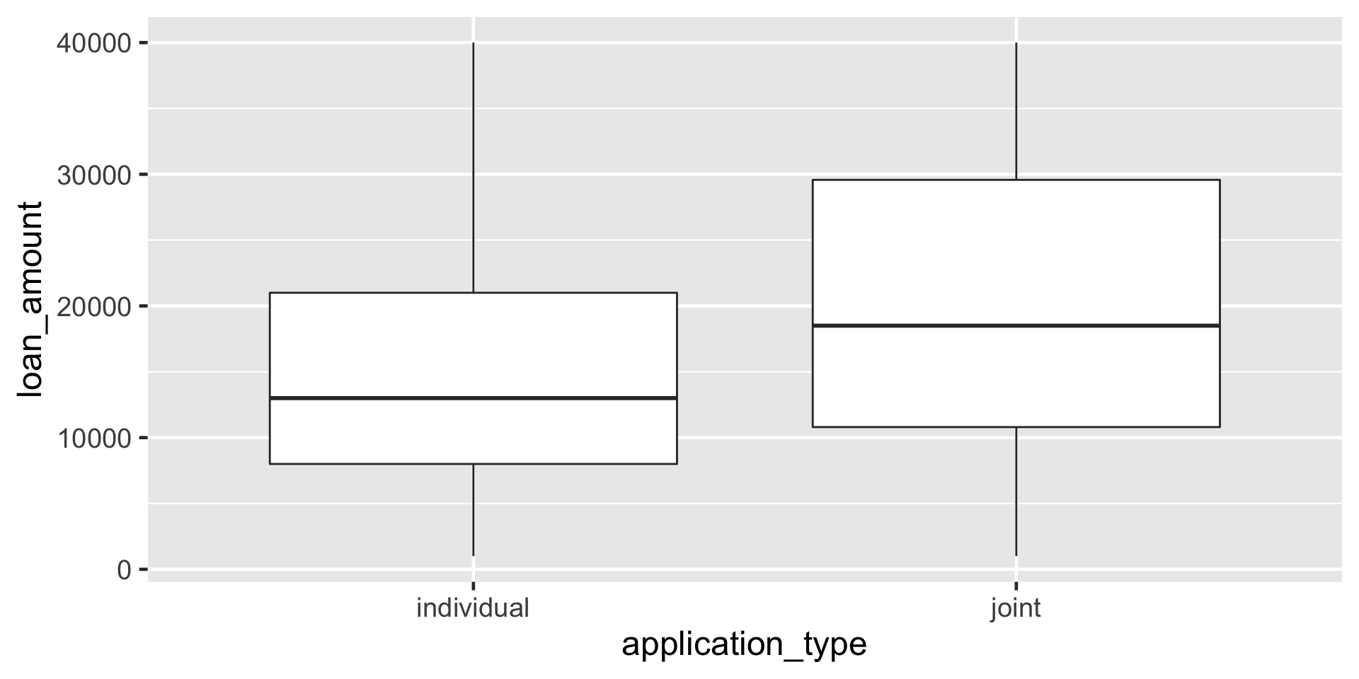
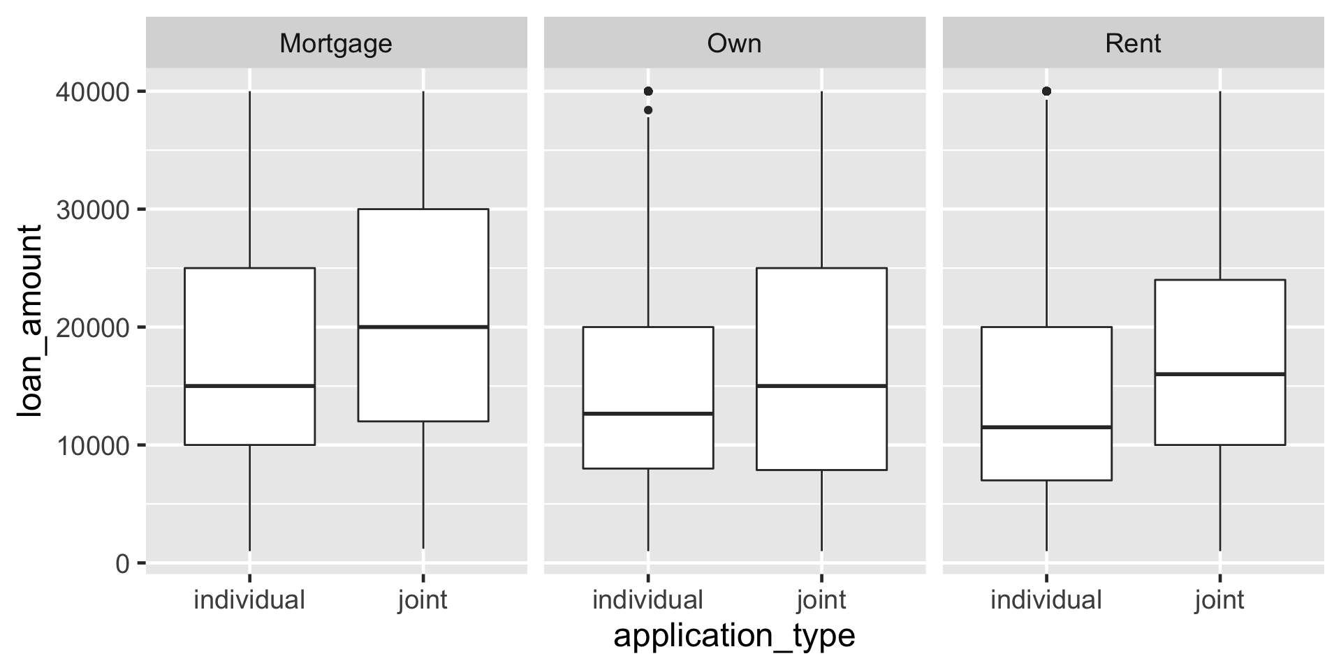
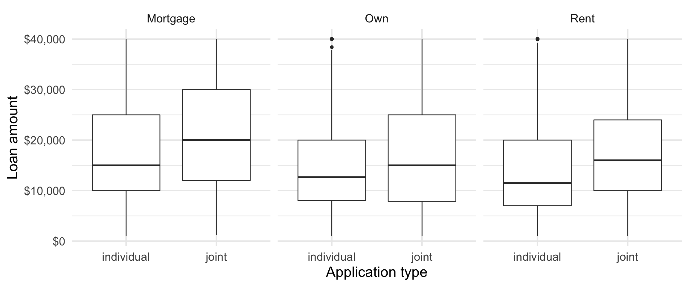
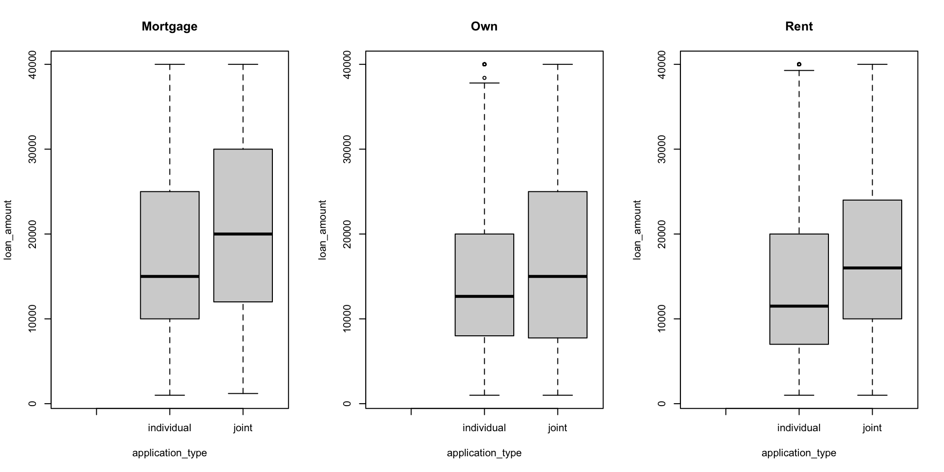
Using the loans data, create side-by-side box plots that shows the relationship between loan amount and application type, faceted by homeownership.

Compare answers with your neighbor and choose an approach you would teach in an intro course. Then, type your chosen answer and some narrative about how you would approach teaching it describing how you would teach it.

See next style for desired output.

10:00

Desired output

Break it down I

Using the loans data, create side-by-side box plots that shows the relationship between annual income and application type, faceted by homeownership.

ggplot(loans)

Break it down II

Using the loans data, create side-by-side box plots that shows the relationship between annual income and application type, faceted by homeownership.

ggplot(loans, 
       aes(x = application_type))

Break it down III

Using the loans data, create side-by-side box plots that shows the relationship between annual income and application type, faceted by homeownership.

ggplot(loans, 
       aes(x = application_type,
           y = loan_amount))

Break it down IV

Using the loans data, create side-by-side box plots that shows the relationship between annual income and application type, faceted by homeownership.

ggplot(loans, 
       aes(x = application_type,
           y = loan_amount)) +
  geom_boxplot()

Break it down IV

Using the loans data, create side-by-side box plots that shows the relationship between annual income and application type, faceted by homeownership.

ggplot(loans, 
       aes(x = application_type,
           y = loan_amount)) +
  geom_boxplot() +
  facet_wrap(~ homeownership)

Plotting with ggplot()

ggplot(loans, 
       aes(x = application_type, y = loan_amount)) +
  geom_boxplot() +
  facet_wrap(~ homeownership)

• Each layer produces a valid plot
• Faceting by a third variable takes only one new function

Plotting with boxplot()

levels <- sort(unique(loans$homeownership))
levels

[1] "Mortgage" "Own"      "Rent"    

loans1 <- loans[loans$homeownership == levels[1],]
loans2 <- loans[loans$homeownership == levels[2],]
loans3 <- loans[loans$homeownership == levels[3],]

Plotting with boxplot()

par(mfrow = c(1, 3))

boxplot(loan_amount ~ application_type, 
        data = loans1, main = levels[1])
boxplot(loan_amount ~ application_type, 
        data = loans2, main = levels[2])
boxplot(loan_amount ~ application_type, 
        data = loans3, main = levels[3])

Visualizing a different relationship

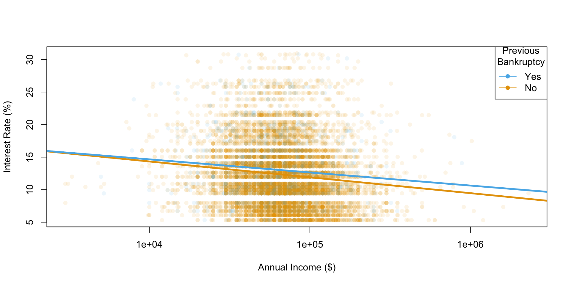
Visualize the relationship between interest rate and annual income, conditioned on whether the applicant had a bankruptcy.

Plotting with ggplot()

ggplot(loans, 
       aes(y = interest_rate, x = annual_income, 
           color = bankruptcy)) +
  geom_point(alpha = 0.1) + 
  geom_smooth(method = "lm", size = 2, se = FALSE) + 
  scale_x_log10()

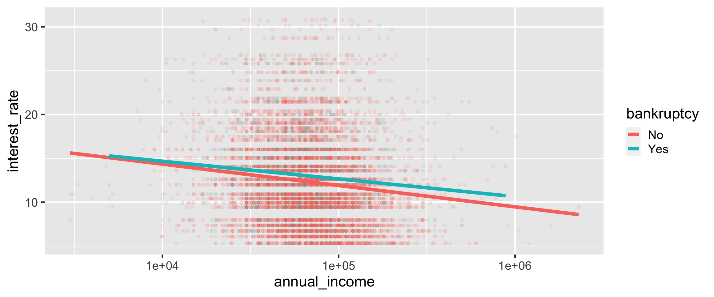
Further customizing ggplot()

ggplot(loans, 
       aes(y = interest_rate, x = annual_income, 
           color = bankruptcy)) +
  geom_point(alpha = 0.1) + 
  geom_smooth(method = "lm", size = 2, se = FALSE) + 
  scale_x_log10(labels = scales::label_dollar()) +
  scale_y_continuous(labels = scales::label_percent(scale = 1)) +
  scale_color_OkabeIto() +
  labs(x = "Annual Income", y = "Interest Rate", 
       color = "Previous\nBankruptcy") +
  theme_minimal(base_size = 18)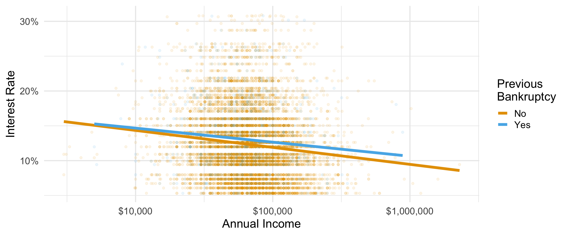

Plotting with plot()

# From the OkabeIto palette
cols = c(No = "#e6a003", Yes = "#57b4e9")

plot(
  loans$annual_income,
  loans$interest_rate,
  pch = 16,
  col = adjustcolor(cols[loans$bankruptcy], alpha.f = 0.1),
  log = "x",
  xlab = "Annual Income ($)",
  ylab = "Interest Rate (%)",
  xaxp = c(1000, 10000000, 1)
)

lm_b_no = lm(
  interest_rate ~ log10(annual_income), 
  data = loans[loans$bankruptcy == "No",]
)
lm_b_yes = lm(
  interest_rate ~ log10(annual_income), 
  data = loans[loans$bankruptcy == "Yes",]
)

abline(lm_b_no, col = cols["No"], lwd = 3)
abline(lm_b_yes, col = cols["Yes"], lwd = 3)

legend(
  "topright", 
  legend = c("Yes", "No"), 
  title = "Previous\nBankruptcy", 
  col = cols[c("Yes", "No")], 
  pch = 16, lwd = 1
)

Plotting with plot()

Beyond wrangling, summaries, visualizations

Modeling and inference with tidymodels:

• A unified interface to modeling functions available in a large variety of packages

• Sticking to the data frame in / data frame out paradigm

• Guardrails for methodology

Next module is teaching with tidymodels!

Pedagogical strengths of the tidyverse

Consistency

• No matter which approach or tool you use, you should strive to be consistent in the classroom whenever possible

• Tidyverse offers consistency, something we believe to be of the utmost importance, allowing students to move knowledge about function arguments to their long-term memory

Teaching consistently

• Challenge: Google and Stack Overflow can be less useful – demo problem solving

• Counter-proposition: teach all (or multiple) syntaxes at once – trying to teach two (or more!) syntaxes at once will slow the pace of the course, introduce unnecessary syntactic confusion, and make it harder for students to complete their work.

• “Disciplined in what we teach, liberal in what we accept”

Postel, J. (1980). DoD standard internet protocol. ACM SIGCOMM Computer Communication Review, 10(4), 12-51. datatracker.ietf.org/doc/html/rfc760

Mixability

• Mix with base R code or code from other packages

• In fact, you can’t not mix with base R code!

Scalability

Adding a new variable to a visualization or a new summary statistic doesn’t require introducing a numerous functions, interfaces, and data structures

User-centered design

• Interfaces designed with user experience (and learning) in mind

• Continuous feedback collection and iterative improvements based on user experiences improve functions’ and packages’ usability (and learnability)

Readability

Interfaces that are designed to produce readable code

Community

• The encouraging and inclusive tidyverse community is one of the benefits of the paradigm

• Each package comes with a website, each of these websites are similarly laid out, and results of example code are displayed, and extensive vignettes describe how to use various functions from the package together

Shared syntax

Get SQL for free with dplyr verbs!

Final thoughts

Building a curriculum

• Start with library(tidyverse)

• Teach by learning goals, not packages

Keeping up with the tidyverse

• Blog posts highlight updates, along with the reasoning behind them and worked examples

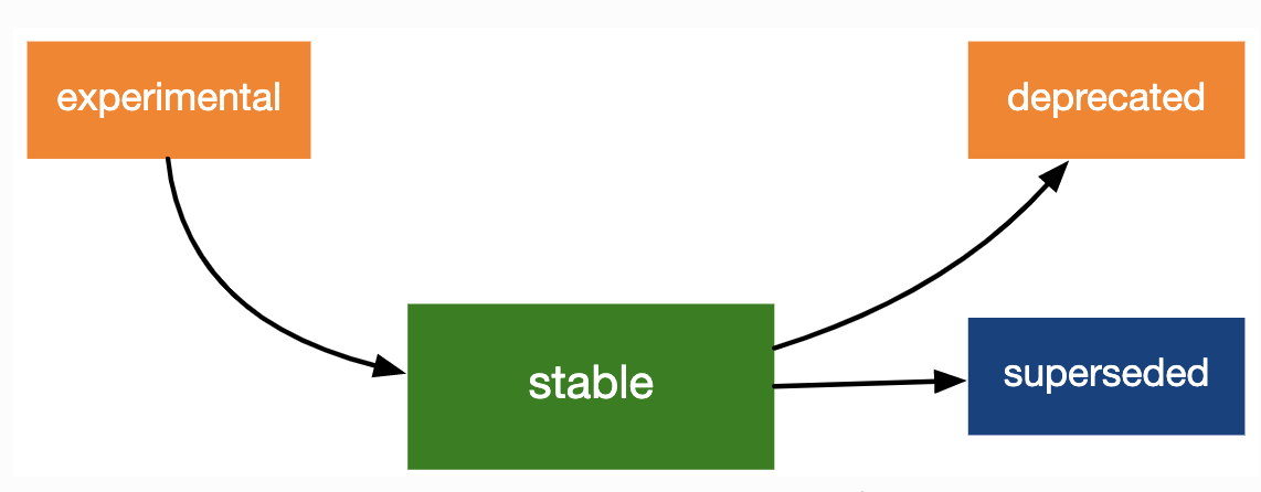
• Lifecycle stages and badges

Coda

We are all converts to the tidyverse and have made a conscious choice to use it in our research and our teaching. We each learned R without the tidyverse and have all spent quite a few years teaching without it at a variety of levels from undergraduate introductory statistics courses to graduate statistical computing courses. This paper is a synthesis of the reasons supporting our tidyverse choice, along with benefits and challenges associated with teaching statistics with the tidyverse.

Çetinkaya-Rundel, M., Hardin, J., Baumer, B. S., McNamara, A., Horton, N. J., & Rundel, C. (2021). An educator’s perspective of the tidyverse. arXiv preprint arXiv:2108.03510. arxiv.org/abs/2108.03510

Discussion

Do you teach with the tidyverse?

• If yes, what are some highlights of your teaching experience and what are some challenges?
• If no, what is your approach and, if you’ve considered the tidyverse but decided against it, why?

Any other discussion points of interest?

Discuss with your partner for a few minutes first, before sharing with the big group.

04:00

Time permitting

Let’s take a look at the source code for these slides for some of the highlighting tricks!