Teaching modern modeling with tidymodels

rstudio::conf(2022)
Designing the data science classroom

Maria Tackett

Session outline

Teaching modern modeling
Introducing tidymodels
Teaching with tidymodels
- Feature engineering
- Prediction + model evaluation
- Train / test data
Putting it all together

Teaching modern modeling

GAISE guidelines

Teach statistical thinking.
- Teach statistics as an investigative process of problem-solving and decision-making.
- Give students experience with multivariable thinking.
Integrate real data with a context and purpose.
Use technology to explore concepts and analyze data.

See Guidelines for Assessment and Instruction in Statistics Education (GAISE) 2016 Report for full report.

Teaching modern regression

Facilitate opportunities for students to…

Regularly engage with real-world applications and complex data
Develop proficiency using professional statistical software and using a reproducible workflow
Identify appropriate methods based on the primary analysis objective - inference or prediction
Develop important non-technical skills, specifically written communication and teamwork

Introducing tidymodels

Tidymodels

The tidymodels framework is a collection of packages for modeling and machine learning using tidyverse principles.

install.packages("tidymodels")

Tidymodels

library(tidymodels)

── Attaching packages ────────────────────────────────────── tidymodels 1.0.0 ──

✔ broom        1.0.0     ✔ rsample      1.0.0
✔ dials        1.0.0     ✔ tune         1.0.0
✔ infer        1.0.2     ✔ workflows    1.0.0
✔ modeldata    1.0.0     ✔ workflowsets 1.0.0
✔ parsnip      1.0.0     ✔ yardstick    1.0.0
✔ recipes      1.0.1

── Conflicts ───────────────────────────────────────── tidymodels_conflicts() ──
✖ scales::discard() masks purrr::discard()
✖ dplyr::filter()   masks stats::filter()
✖ recipes::fixed()  masks stringr::fixed()
✖ dplyr::lag()      masks stats::lag()
✖ yardstick::spec() masks readr::spec()
✖ recipes::step()   masks stats::step()
• Learn how to get started at https://www.tidymodels.org/start/

Data: Loans from Lending Club

The data is the loans_full_schema data set from the openintro package and featured in the OpenIntro textbooks . It contains information about 50,000 loans made through the Lending Club platform. The variables we’ll use in this presentation are

interest_rate: Interest rate of the loan the applicant received.
debt_to_income: Debt-to-income ratio.
term: The number of months of the loan the applicant received.
delinq_2y: Number of delinquencies on lines of credit in the last 2 years.

Data: Loans from Lending Club

library(openintro)
glimpse(loans_full_schema)

Rows: 10,000
Columns: 55
$ emp_title                        <chr> "global config engineer ", "warehouse…
$ emp_length                       <dbl> 3, 10, 3, 1, 10, NA, 10, 10, 10, 3, 1…
$ state                            <fct> NJ, HI, WI, PA, CA, KY, MI, AZ, NV, I…
$ homeownership                    <fct> MORTGAGE, RENT, RENT, RENT, RENT, OWN…
$ annual_income                    <dbl> 90000, 40000, 40000, 30000, 35000, 34…
$ verified_income                  <fct> Verified, Not Verified, Source Verifi…
$ debt_to_income                   <dbl> 18.01, 5.04, 21.15, 10.16, 57.96, 6.4…
$ annual_income_joint              <dbl> NA, NA, NA, NA, 57000, NA, 155000, NA…
$ verification_income_joint        <fct> , , , , Verified, , Not Verified, , ,…
$ debt_to_income_joint             <dbl> NA, NA, NA, NA, 37.66, NA, 13.12, NA,…
$ delinq_2y                        <int> 0, 0, 0, 0, 0, 1, 0, 1, 1, 0, 0, 0, 0…
$ months_since_last_delinq         <int> 38, NA, 28, NA, NA, 3, NA, 19, 18, NA…
$ earliest_credit_line             <dbl> 2001, 1996, 2006, 2007, 2008, 1990, 2…
$ inquiries_last_12m               <int> 6, 1, 4, 0, 7, 6, 1, 1, 3, 0, 4, 4, 8…
$ total_credit_lines               <int> 28, 30, 31, 4, 22, 32, 12, 30, 35, 9,…
$ open_credit_lines                <int> 10, 14, 10, 4, 16, 12, 10, 15, 21, 6,…
$ total_credit_limit               <int> 70795, 28800, 24193, 25400, 69839, 42…
$ total_credit_utilized            <int> 38767, 4321, 16000, 4997, 52722, 3898…
$ num_collections_last_12m         <int> 0, 0, 0, 0, 0, 0, 0, 0, 0, 0, 0, 0, 0…
$ num_historical_failed_to_pay     <int> 0, 1, 0, 1, 0, 0, 0, 0, 0, 0, 1, 0, 0…
$ months_since_90d_late            <int> 38, NA, 28, NA, NA, 60, NA, 71, 18, N…
$ current_accounts_delinq          <int> 0, 0, 0, 0, 0, 0, 0, 0, 0, 0, 0, 0, 0…
$ total_collection_amount_ever     <int> 1250, 0, 432, 0, 0, 0, 0, 0, 0, 0, 0,…
$ current_installment_accounts     <int> 2, 0, 1, 1, 1, 0, 2, 2, 6, 1, 2, 1, 2…
$ accounts_opened_24m              <int> 5, 11, 13, 1, 6, 2, 1, 4, 10, 5, 6, 7…
$ months_since_last_credit_inquiry <int> 5, 8, 7, 15, 4, 5, 9, 7, 4, 17, 3, 4,…
$ num_satisfactory_accounts        <int> 10, 14, 10, 4, 16, 12, 10, 15, 21, 6,…
$ num_accounts_120d_past_due       <int> 0, 0, 0, 0, 0, 0, 0, NA, 0, 0, 0, 0, …
$ num_accounts_30d_past_due        <int> 0, 0, 0, 0, 0, 0, 0, 0, 0, 0, 0, 0, 0…
$ num_active_debit_accounts        <int> 2, 3, 3, 2, 10, 1, 3, 5, 11, 3, 2, 2,…
$ total_debit_limit                <int> 11100, 16500, 4300, 19400, 32700, 272…
$ num_total_cc_accounts            <int> 14, 24, 14, 3, 20, 27, 8, 16, 19, 7, …
$ num_open_cc_accounts             <int> 8, 14, 8, 3, 15, 12, 7, 12, 14, 5, 8,…
$ num_cc_carrying_balance          <int> 6, 4, 6, 2, 13, 5, 6, 10, 14, 3, 5, 3…
$ num_mort_accounts                <int> 1, 0, 0, 0, 0, 3, 2, 7, 2, 0, 2, 3, 3…
$ account_never_delinq_percent     <dbl> 92.9, 100.0, 93.5, 100.0, 100.0, 78.1…
$ tax_liens                        <int> 0, 0, 0, 1, 0, 0, 0, 0, 0, 0, 0, 0, 0…
$ public_record_bankrupt           <int> 0, 1, 0, 0, 0, 0, 0, 0, 0, 0, 1, 0, 0…
$ loan_purpose                     <fct> moving, debt_consolidation, other, de…
$ application_type                 <fct> individual, individual, individual, i…
$ loan_amount                      <int> 28000, 5000, 2000, 21600, 23000, 5000…
$ term                             <dbl> 60, 36, 36, 36, 36, 36, 60, 60, 36, 3…
$ interest_rate                    <dbl> 14.07, 12.61, 17.09, 6.72, 14.07, 6.7…
$ installment                      <dbl> 652.53, 167.54, 71.40, 664.19, 786.87…
$ grade                            <fct> C, C, D, A, C, A, C, B, C, A, C, B, C…
$ sub_grade                        <fct> C3, C1, D1, A3, C3, A3, C2, B5, C2, A…
$ issue_month                      <fct> Mar-2018, Feb-2018, Feb-2018, Jan-201…
$ loan_status                      <fct> Current, Current, Current, Current, C…
$ initial_listing_status           <fct> whole, whole, fractional, whole, whol…
$ disbursement_method              <fct> Cash, Cash, Cash, Cash, Cash, Cash, C…
$ balance                          <dbl> 27015.86, 4651.37, 1824.63, 18853.26,…
$ paid_total                       <dbl> 1999.330, 499.120, 281.800, 3312.890,…
$ paid_principal                   <dbl> 984.14, 348.63, 175.37, 2746.74, 1569…
$ paid_interest                    <dbl> 1015.19, 150.49, 106.43, 566.15, 754.…
$ paid_late_fees                   <dbl> 0, 0, 0, 0, 0, 0, 0, 0, 0, 0, 0, 0, 0…

Exploratory data analysis

ggplot(loans_full_schema, aes(x = interest_rate)) +
  geom_histogram(binwidth = 1) +
  labs(
    x = "Interest rate", y = "Count",
    title = "Distribution of loan interest rates"
  )

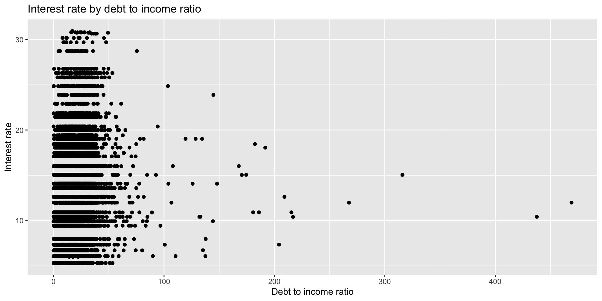
Exploratory data analysis

ggplot(data = loans_full_schema, aes(x = debt_to_income, y = interest_rate )) +
  geom_point() + 
  labs(x = "Debt to income ratio", y = "Interest rate", 
       title = "Interest rate by debt to income ratio")

Exploratory data analysis

ggplot(data = loans_full_schema, aes(x = interest_rate, fill = factor(term))) +
  geom_density(alpha= 0.5) + 
  labs(x = "Interest rate", y = "Density", 
       fill = "Term (in months)",
       title = "Interest rate by debt by term length")

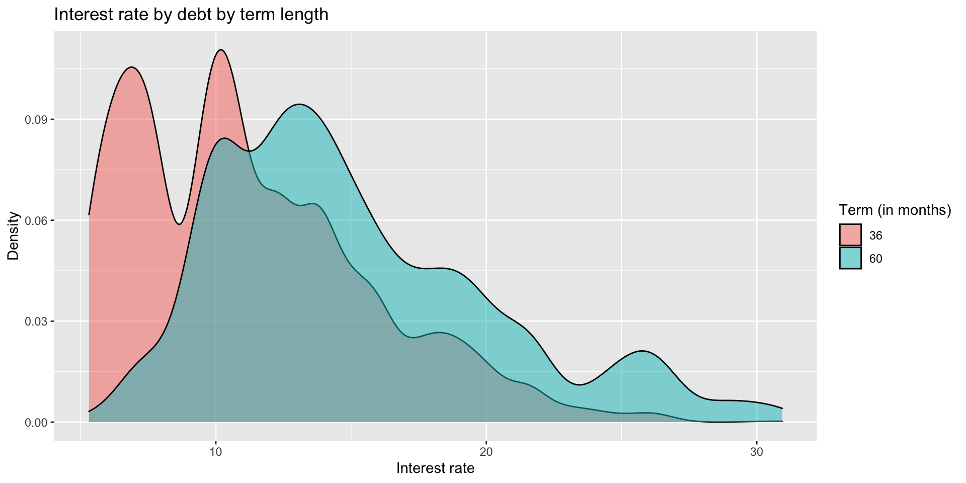
Regression syntax

Fit a linear regression model to predict the interest rate using the debt to income ratio.

Base R
Tidymodels

base_lm <- lm(interest_rate ~ debt_to_income, data = loans_full_schema)
summary(base_lm)


Call:
lm(formula = interest_rate ~ debt_to_income, data = loans_full_schema)

Residuals:
     Min       1Q   Median       3Q      Max 
-21.7391  -3.7203  -0.7945   2.7351  18.6274 

Coefficients:
                Estimate Std. Error t value Pr(>|t|)    
(Intercept)    11.511445   0.080732  142.59   <2e-16 ***
debt_to_income  0.047183   0.003302   14.29   <2e-16 ***
---
Signif. codes:  0 '***' 0.001 '**' 0.01 '*' 0.05 '.' 0.1 ' ' 1

Residual standard error: 4.948 on 9974 degrees of freedom
  (24 observations deleted due to missingness)
Multiple R-squared:  0.02007,   Adjusted R-squared:  0.01997 
F-statistic: 204.2 on 1 and 9974 DF,  p-value: < 2.2e-16

tidy_lm <- linear_reg() |> 
  set_engine("lm") |>
  fit(interest_rate ~ debt_to_income, data = loans_full_schema)

tidy(tidy_lm)

# A tibble: 2 × 5
  term           estimate std.error statistic  p.value
  <chr>             <dbl>     <dbl>     <dbl>    <dbl>
1 (Intercept)     11.5      0.0807      143.  0       
2 debt_to_income   0.0472   0.00330      14.3 7.05e-46

Model summaries using broom

Can utilize functions from the broom package to produce tidy summaries of models fit using Base R or the tidymodels framework

tidy(): summarizes information about model components
glance(): reports information about the entire model
augment(): adds information about observations to a data set

base_lm <- lm(interest_rate ~ debt_to_income, data = loans_full_schema)
tidy(base_lm)

# A tibble: 2 × 5
  term           estimate std.error statistic  p.value
  <chr>             <dbl>     <dbl>     <dbl>    <dbl>
1 (Intercept)     11.5      0.0807      143.  0       
2 debt_to_income   0.0472   0.00330      14.3 7.05e-46

tidy_lm <- linear_reg() |> 
  set_engine("lm") |>
  fit(interest_rate ~ debt_to_income, data = loans_full_schema)
tidy(tidy_lm)

# A tibble: 2 × 5
  term           estimate std.error statistic  p.value
  <chr>             <dbl>     <dbl>     <dbl>    <dbl>
1 (Intercept)     11.5      0.0807      143.  0       
2 debt_to_income   0.0472   0.00330      14.3 7.05e-46

`glance()`

Base R
Tidymodels

glance(base_lm)

# A tibble: 1 × 12
  r.squared adj.r.s…¹ sigma stati…²  p.value    df  logLik    AIC    BIC devia…³
      <dbl>     <dbl> <dbl>   <dbl>    <dbl> <dbl>   <dbl>  <dbl>  <dbl>   <dbl>
1    0.0201    0.0200  4.95    204. 7.05e-46     1 -30105. 60217. 60238. 244166.
# … with 2 more variables: df.residual <int>, nobs <int>, and abbreviated
#   variable names ¹adj.r.squared, ²statistic, ³deviance
# ℹ Use `colnames()` to see all variable names

glance(tidy_lm)

# A tibble: 1 × 12
  r.squared adj.r.s…¹ sigma stati…²  p.value    df  logLik    AIC    BIC devia…³
      <dbl>     <dbl> <dbl>   <dbl>    <dbl> <dbl>   <dbl>  <dbl>  <dbl>   <dbl>
1    0.0201    0.0200  4.95    204. 7.05e-46     1 -30105. 60217. 60238. 244166.
# … with 2 more variables: df.residual <int>, nobs <int>, and abbreviated
#   variable names ¹adj.r.squared, ²statistic, ³deviance
# ℹ Use `colnames()` to see all variable names

`augment()`

Base R
Tidymodels

base_lm_aug <- augment(base_lm)
base_lm_aug

# A tibble: 9,976 × 9
   .rownames interest_rate debt_…¹ .fitted .resid    .hat .sigma .cooksd .std.…²
   <chr>             <dbl>   <dbl>   <dbl>  <dbl>   <dbl>  <dbl>   <dbl>   <dbl>
 1 1                 14.1    18.0     12.4  1.71  1.01e-4   4.95 6.02e-6  0.345 
 2 2                 12.6     5.04    11.7  0.861 1.91e-4   4.95 2.89e-6  0.174 
 3 3                 17.1    21.2     12.5  4.58  1.02e-4   4.95 4.36e-5  0.926 
 4 4                  6.72   10.2     12.0 -5.27  1.38e-4   4.95 7.80e-5 -1.07  
 5 5                 14.1    58.0     14.2 -0.176 7.65e-4   4.95 4.86e-7 -0.0356
 6 6                  6.72    6.46    11.8 -5.10  1.74e-4   4.95 9.22e-5 -1.03  
 7 7                 13.6    23.7     12.6  0.962 1.09e-4   4.95 2.06e-6  0.194 
 8 8                 12.0    16.2     12.3 -0.285 1.05e-4   4.95 1.74e-7 -0.0577
 9 9                 13.6    36.5     13.2  0.357 2.32e-4   4.95 6.04e-7  0.0722
10 10                 6.71   18.9     12.4 -5.69  1.00e-4   4.95 6.64e-5 -1.15  
# … with 9,966 more rows, and abbreviated variable names ¹debt_to_income,
#   ².std.resid
# ℹ Use `print(n = ...)` to see more rows

tidy_lm_aug <- augment(tidy_lm$fit)
tidy_lm_aug

# A tibble: 9,976 × 9
   .rownames interest_rate debt_…¹ .fitted .resid    .hat .sigma .cooksd .std.…²
   <chr>             <dbl>   <dbl>   <dbl>  <dbl>   <dbl>  <dbl>   <dbl>   <dbl>
 1 1                 14.1    18.0     12.4  1.71  1.01e-4   4.95 6.02e-6  0.345 
 2 2                 12.6     5.04    11.7  0.861 1.91e-4   4.95 2.89e-6  0.174 
 3 3                 17.1    21.2     12.5  4.58  1.02e-4   4.95 4.36e-5  0.926 
 4 4                  6.72   10.2     12.0 -5.27  1.38e-4   4.95 7.80e-5 -1.07  
 5 5                 14.1    58.0     14.2 -0.176 7.65e-4   4.95 4.86e-7 -0.0356
 6 6                  6.72    6.46    11.8 -5.10  1.74e-4   4.95 9.22e-5 -1.03  
 7 7                 13.6    23.7     12.6  0.962 1.09e-4   4.95 2.06e-6  0.194 
 8 8                 12.0    16.2     12.3 -0.285 1.05e-4   4.95 1.74e-7 -0.0577
 9 9                 13.6    36.5     13.2  0.357 2.32e-4   4.95 6.04e-7  0.0722
10 10                 6.71   18.9     12.4 -5.69  1.00e-4   4.95 6.64e-5 -1.15  
# … with 9,966 more rows, and abbreviated variable names ¹debt_to_income,
#   ².std.resid
# ℹ Use `print(n = ...)` to see more rows

Why Tidymodels?

There are advantages for more advanced modeling:

Consistent syntax for different model types (linear, logistic, random forest, Bayesian, etc.)
Streamline modeling workflow
- Split data into train and test sets
- Transform and create new variables
- Assess model performance
- Use model for prediction and inference

Teaching with tidymodels

Tidymodels syntax

linear_reg() |> 
  set_engine("lm") |>
  fit(interest_rate ~ debt_to_income, data = loans_full_schema) |>
  tidy()

# A tibble: 2 × 5
  term           estimate std.error statistic  p.value
  <chr>             <dbl>     <dbl>     <dbl>    <dbl>
1 (Intercept)     11.5      0.0807      143.  0       
2 debt_to_income   0.0472   0.00330      14.3 7.05e-46

Let’s break down the syntax.

1️⃣ Specify model

linear_reg()

Linear Regression Model Specification (regression)

Computational engine: lm

2️⃣ Set computational engine

linear_reg() |> 
  set_engine("lm")

Linear Regression Model Specification (regression)

Computational engine: lm

3️⃣ Fit the model

linear_reg() |> 
  set_engine("lm") |>
  fit(interest_rate ~ debt_to_income, data = loans_full_schema)

parsnip model object


Call:
stats::lm(formula = interest_rate ~ debt_to_income, data = data)

Coefficients:
   (Intercept)  debt_to_income  
      11.51145         0.04718

4️⃣ Summarize output

linear_reg() |> 
  set_engine("lm") |>
  fit(interest_rate ~ debt_to_income, data = loans_full_schema) |>
  tidy()

# A tibble: 2 × 5
  term           estimate std.error statistic  p.value
  <chr>             <dbl>     <dbl>     <dbl>    <dbl>
1 (Intercept)     11.5      0.0807      143.  0       
2 debt_to_income   0.0472   0.00330      14.3 7.05e-46

Consistent syntax for other models

The syntax is the same if we fit a more advanced model, such as a logistic regression model.

Fit a model to predict the loan term length (36 or 60 months) based on the loan amount.

logistic_reg() |>
  set_engine("glm") |>
  fit(factor(term) ~ loan_amount, data = loans_full_schema) |>
  tidy()

# A tibble: 2 × 5
  term          estimate  std.error statistic   p.value
  <chr>            <dbl>      <dbl>     <dbl>     <dbl>
1 (Intercept) -2.28      0.0493         -46.2 0        
2 loan_amount  0.0000814 0.00000232      35.1 1.02e-269

Feature engineering

Feature engineering is the process of transforming raw variables in preparation for use in a statistical model.
You may be familiar doing feature engineering using dplyr before fitting the model.
The recipes package makes it possible to do feature engineering as part of the modeling workflow using “dplyr-like” functions.

Example: Predicting interest rate

Goal: Fit a model to predict the interest rate based on the term, debt to income ratio, and number of delinquencies in the past two years.
We need to do the following to prepare the predictors for the model:
- Make term a factor.
- Mean-center debt_to_income.
- Split delinq_2y into the categories 0, 1, 2, 3+.

Feature engineering using dplyr

# Feature engineering
loans_full_schema <- loans_full_schema |>
  mutate(term_fct = as_factor(term)) |>
  mutate(debt_to_income_cent = 
           debt_to_income - mean(debt_to_income, na.rm = TRUE)) |>
  mutate(delinq_2y_cat = 
           cut(delinq_2y, breaks = c(-Inf,0,1, 2, 3, Inf)))

# Fit the model 
lm(interest_rate ~ term_fct + debt_to_income_cent + delinq_2y_cat,
   data = loans_full_schema) |>
  tidy()

# A tibble: 7 × 5
  term                  estimate std.error statistic   p.value
  <chr>                    <dbl>     <dbl>     <dbl>     <dbl>
1 (Intercept)            11.0      0.0584     189.   0        
2 term_fct60              3.86     0.100       38.5  6.67e-303
3 debt_to_income_cent     0.0429   0.00307     14.0  5.47e- 44
4 delinq_2y_cat(0,1]      1.37     0.153        8.95 4.08e- 19
5 delinq_2y_cat(1,2]      1.68     0.291        5.76 8.57e-  9
6 delinq_2y_cat(2,3]      2.46     0.492        5.00 5.78e-  7
7 delinq_2y_cat(3, Inf]   2.85     0.563        5.05 4.39e-  7

Discussion

What is a disadvantage to this approach?

02:00

Feature engineering with recipes

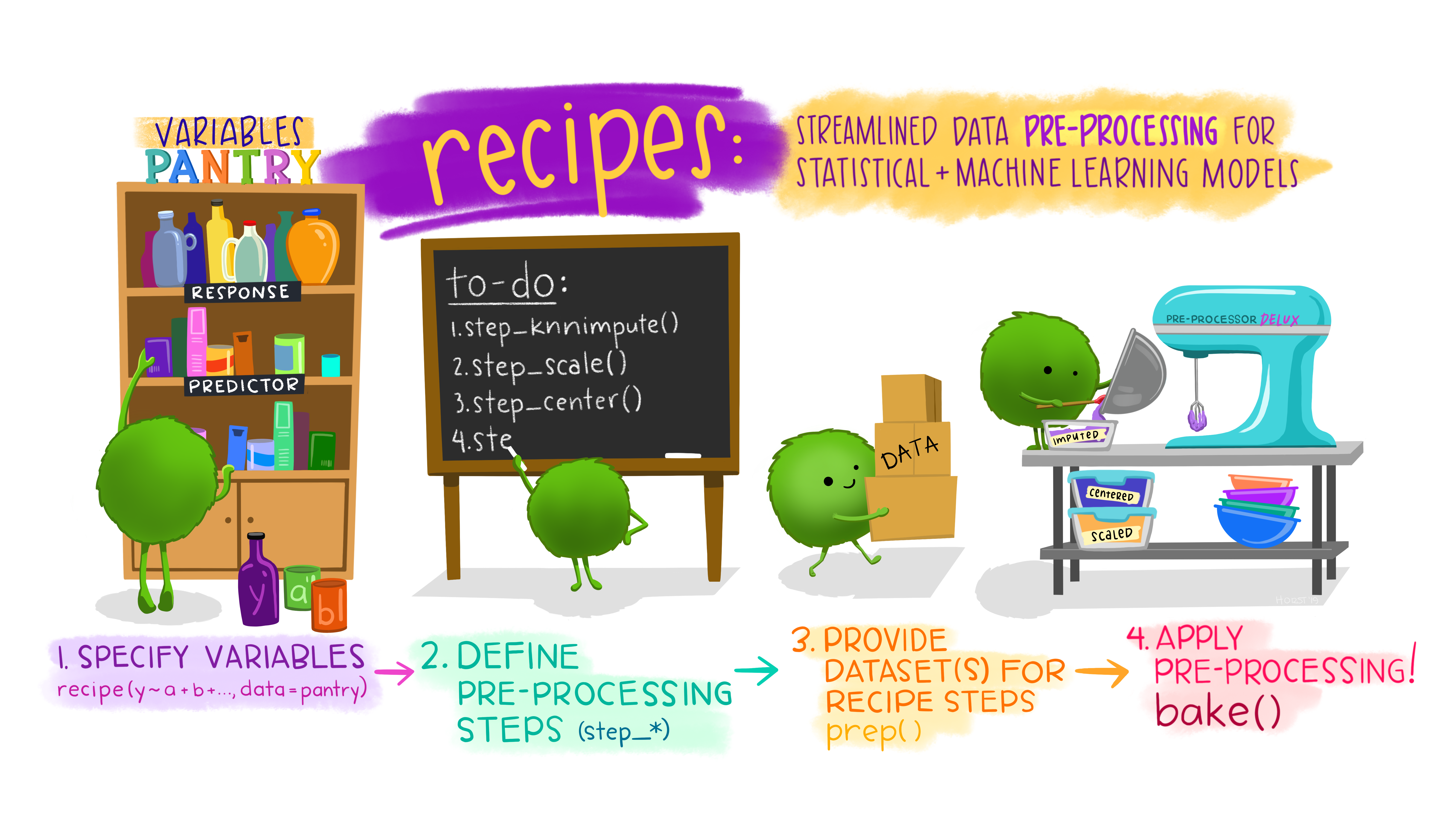
Illustration by Allison Horst

Specify the variables

interest_rec <- recipe(
  interest_rate ~ term + debt_to_income + delinq_2y, 
  data = loans_full_schema 
  )

interest_rec

Recipe

Inputs:

      role #variables
   outcome          1
 predictor          3

Define pre-processing steps

Make term a factor.

interest_rec <- interest_rec |>
  step_mutate(term = as_factor(term))

interest_rec

Recipe

Inputs:

      role #variables
   outcome          1
 predictor          3

Operations:

Variable mutation for as_factor(term)

Define pre-processing steps

Mean-center debt_to_income.

interest_rec <- interest_rec |>
  step_center(debt_to_income)

interest_rec

Recipe

Inputs:

      role #variables
   outcome          1
 predictor          3

Operations:

Variable mutation for as_factor(term)
Centering for debt_to_income

Define pre-processing steps

Break delinq_2y into the categories 0, 1, 2, 3+.

interest_rec <- interest_rec |>
  step_cut(delinq_2y, breaks = c(-Inf,0,1, 2, 3, Inf))

interest_rec

Recipe

Inputs:

      role #variables
   outcome          1
 predictor          3

Operations:

Variable mutation for as_factor(term)
Centering for debt_to_income
Cut numeric for delinq_2y

Putting it all together

interest_rec <- recipe(interest_rate ~ term + debt_to_income + delinq_2y,
                       data = loans_full_schema) |>
  step_mutate(term = as_factor(term))|>
  step_center(debt_to_income) |>
  step_cut(delinq_2y, breaks = c(-Inf,0,1, 2, 3, Inf))

Putting it all together

interest_rec

Recipe

Inputs:

      role #variables
   outcome          1
 predictor          3

Operations:

Variable mutation for as_factor(term)
Centering for debt_to_income
Cut numeric for delinq_2y

Prep and bake to see created variables

interest_rec |>
  prep()|>
  bake(loans_full_schema) |>
  head()

# A tibble: 6 × 4
  term  debt_to_income delinq_2y interest_rate
  <fct>          <dbl> <fct>             <dbl>
1 60             -1.30 [-Inf,0]          14.1 
2 36            -14.3  [-Inf,0]          12.6 
3 36              1.84 [-Inf,0]          17.1 
4 36             -9.15 [-Inf,0]           6.72
5 36             38.7  [-Inf,0]          14.1 
6 36            -12.8  (0,1]              6.72

Exercise 1: Feature engineering

RStudio Cloud > “Model 3 - Tidymodels” > ex-3-1.qmd

Write the recipe for the model in the exercise file. Call the recipe loans_rec. Use the appropriate step_* functions to complete the feature engineering steps shown in the dplyr pipeline.

You can find the list of step_* functions on the recipes reference page.

15:00

Fit the model using `workflow()`

Workflows bring together models and recipes, making them easier to apply to multiple data sets, e.g, training and test data.

Specify the model

interest_spec <- linear_reg() |>
  set_engine("lm")

Build workflow

interest_workflow <- workflow() |>
  add_model(interest_spec) |>
  add_recipe(interest_rec)

View workflow

interest_workflow

══ Workflow ════════════════════════════════════════════════════════════════════
Preprocessor: Recipe
Model: linear_reg()

── Preprocessor ────────────────────────────────────────────────────────────────
3 Recipe Steps

• step_mutate()
• step_center()
• step_cut()

── Model ───────────────────────────────────────────────────────────────────────
Linear Regression Model Specification (regression)

Computational engine: lm

Fit model to data

interest_fit <- interest_workflow %>%
  fit(data = loans_full_schema)

tidy(interest_fit)

# A tibble: 7 × 5
  term              estimate std.error statistic   p.value
  <chr>                <dbl>     <dbl>     <dbl>     <dbl>
1 (Intercept)        11.0      0.0584     189.   0        
2 term60              3.86     0.100       38.5  6.67e-303
3 debt_to_income      0.0429   0.00307     14.0  5.47e- 44
4 delinq_2y(0,1]      1.37     0.153        8.95 4.08e- 19
5 delinq_2y(1,2]      1.68     0.291        5.76 8.57e-  9
6 delinq_2y(2,3]      2.46     0.492        5.00 5.78e-  7
7 delinq_2y(3, Inf]   2.85     0.563        5.05 4.39e-  7

Prediction + Model evaluation

Make predictions

interest_pred <- predict(interest_fit, loans_full_schema) |> 
  bind_cols(loans_full_schema |> select(interest_rate))

interest_pred

# A tibble: 10,000 × 2
   .pred interest_rate
   <dbl>         <dbl>
 1  14.8         14.1 
 2  10.4         12.6 
 3  11.1         17.1 
 4  10.6          6.72
 5  12.7         14.1 
 6  11.8          6.72
 7  15.1         13.6 
 8  16.1         12.0 
 9  13.1         13.6 
10  11.0          6.71
# … with 9,990 more rows
# ℹ Use `print(n = ...)` to see more rows

Model evaluation: \(R^2\)

\(R^2\) is the percent of variability in the interest rate explained by the model.

rsq(interest_pred, truth = interest_rate, estimate = .pred)

# A tibble: 1 × 3
  .metric .estimator .estimate
  <chr>   <chr>          <dbl>
1 rsq     standard       0.157

Model evaluation: \(RMSE\)

\(RMSE\) is a measure of the error in the model predictions.

\[ RMSE = \sqrt{\frac{\sum_{i=1}^{n}(\hat{y}_i - y_i)^2}{n}} \]

rmse(interest_pred, truth = interest_rate, estimate = .pred)

# A tibble: 1 × 3
  .metric .estimator .estimate
  <chr>   <chr>          <dbl>
1 rmse    standard        4.59

Exercise 2: Fit, predict, evaluate

RStudio Cloud > “Model 3 - Tidymodels” > ex-3-2.qmd

Build a workflow and fit the model specified in the exercise. Then calculate predictions and evaluate the model using \(R^2\) and \(RMSE\).

10:00

What is a limitation to the model evaluation we’ve done thus far?

Splitting the data

Splitting the data into training and testing sets allows us to evaluate the model on new data.

Split the data.

set.seed(0725) #to get same split each run
loans_split <- initial_split(loans_full_schema, prop = 0.8) #80% training

Save the training data.

loans_train <- training(loans_split)
dim(loans_train)

[1] 8000   58

Save test data.

loans_test <- testing(loans_split)
dim(loans_test)

[1] 2000   58

Fit the model to the training data

We can fit the model specified in interest_workflow (model spec + recipe) to the training data.

interest_train_fit <- interest_workflow |>
  fit(data = loans_train)

tidy(interest_train_fit)

# A tibble: 7 × 5
  term              estimate std.error statistic   p.value
  <chr>                <dbl>     <dbl>     <dbl>     <dbl>
1 (Intercept)        11.0      0.0646     170.   0        
2 term60              3.91     0.112       35.1  1.05e-250
3 debt_to_income      0.0402   0.00331     12.2  1.12e- 33
4 delinq_2y(0,1]      1.33     0.171        7.79 7.77e- 15
5 delinq_2y(1,2]      1.75     0.323        5.41 6.38e-  8
6 delinq_2y(2,3]      2.48     0.536        4.63 3.79e-  6
7 delinq_2y(3, Inf]   3.01     0.617        4.88 1.09e-  6

Evaluate performance on training data

Calculate predictions

interest_train_pred <- predict(interest_train_fit, loans_train) |> 
  bind_cols(loans_train |> select(interest_rate))

Evaluate model

rsq(interest_train_pred, truth = interest_rate, estimate = .pred)

# A tibble: 1 × 3
  .metric .estimator .estimate
  <chr>   <chr>          <dbl>
1 rsq     standard       0.161

rmse(interest_train_pred, truth = interest_rate, estimate = .pred)

# A tibble: 1 × 3
  .metric .estimator .estimate
  <chr>   <chr>          <dbl>
1 rmse    standard        4.55

Evaluate performance on testing data

Calculate predictions

interest_test_pred <- predict(interest_train_fit, loans_test) |> 
  bind_cols(loans_test |> select(interest_rate))

Evaluate model

rsq(interest_test_pred, truth = interest_rate, estimate = .pred)

# A tibble: 1 × 3
  .metric .estimator .estimate
  <chr>   <chr>          <dbl>
1 rsq     standard       0.140

rmse(interest_test_pred, truth = interest_rate, estimate = .pred)

# A tibble: 1 × 3
  .metric .estimator .estimate
  <chr>   <chr>          <dbl>
1 rmse    standard        4.73

Exercise 3: Train / test data (time permitting)

RStudio Cloud > “Model 3 - Tidymodels” > ex-3-3.qmd

Complete the code below to split the data into training (80%) and testing (20%) sets. Fit the model to the training set, then evaluate the model on the training and test sets.

10:00

Putting it all together

Let’s take a look at a full analysis.

RStudio Cloud > “Model 3 - Tidymodels” > ex-3-full-analysis.qmd

Discussion

Discuss the following with your neighbor.

What is something from this module you can implement in your data science course?
Do you anticipate any challenges / is there anything that makes you hesitant about teaching modeling using tidymodels?

Any other discussion points of interest?

04:00

Teaching modern modeling with tidymodels

Session outline

Teaching modern modeling

GAISE guidelines

Teaching modern regression

Introducing tidymodels

Tidymodels

Tidymodels

Data: Loans from Lending Club

Data: Loans from Lending Club

Exploratory data analysis

Exploratory data analysis

Exploratory data analysis

Regression syntax

Model summaries using broom

tidy()

glance()

augment()

Why Tidymodels?

Teaching with tidymodels

Tidymodels syntax

1️⃣ Specify model

2️⃣ Set computational engine

3️⃣ Fit the model

4️⃣ Summarize output

Consistent syntax for other models

Feature engineering

Example: Predicting interest rate

Feature engineering using dplyr

Discussion

Feature engineering with recipes

Specify the variables

Define pre-processing steps

Define pre-processing steps

Define pre-processing steps

Putting it all together

Putting it all together

Prep and bake to see created variables

Exercise 1: Feature engineering

Fit the model using workflow()

View workflow

Fit model to data

Prediction + Model evaluation

Make predictions

Model evaluation: \(R^2\)

Model evaluation: \(RMSE\)

Exercise 2: Fit, predict, evaluate

What is a limitation to the model evaluation we’ve done thus far?

Splitting the data

Fit the model to the training data

Evaluate performance on training data

Evaluate performance on testing data

Exercise 3: Train / test data (time permitting)

Putting it all together

Discussion

`tidy()`

`glance()`

`augment()`

Fit the model using `workflow()`