The ussie pckage is designed as a teaching example for a course, Building Tidy Tools. In this course, a student will build this package. For each file, they will start with templated functions; they will edit the file themselves, according to the particular exercise.
When a student has a function working the way they want it to work, they will add an exampe in this vignette. What follows is Ian’s attempt to go through the exercise.
library(ussie)
library(dplyr)
#>
#> Attaching package: 'dplyr'
#> The following objects are masked from 'package:stats':
#>
#>     filter, lag
#> The following objects are masked from 'package:base':
#>
#>     intersect, setdiff, setequal, union

conflicted::conflict_prefer("filter", "dplyr")
#> [conflicted] Will prefer dplyr::filter over any other package
You can use the ussie package to work with data for league-play matches for European Football Leagues. The data is provided by James Curley’s engsoccerdata package: the CRAN version has results through summer 2016; the GitHub version has more-recent results.
Get match results
To find out which leagues are available, use uss_countries():
uss_countries()
#> [1] "england" "germany" "holland" "italy"   "spain"
To get the data for a given league, use uss_get_matches() with the country:
uss_get_matches("england")
#> # A tibble: 192,004 × 8
#>    country tier  season date       home         visitor goals_home goals_visitor
#>    <chr>   <fct>  <int> <date>     <chr>        <chr>        <int>         <int>
#>  1 England 1       1888 1888-12-15 Accrington … Aston …          1             1
#>  2 England 1       1888 1889-01-19 Accrington … Blackb…          0             2
#>  3 England 1       1888 1889-03-23 Accrington … Bolton…          2             3
#>  4 England 1       1888 1888-12-01 Accrington … Burnley          5             1
#>  5 England 1       1888 1888-10-13 Accrington … Derby …          6             2
#>  6 England 1       1888 1888-12-29 Accrington … Everton          3             1
#>  7 England 1       1888 1889-01-26 Accrington … Notts …          1             2
#>  8 England 1       1888 1888-10-20 Accrington … Presto…          0             0
#>  9 England 1       1888 1889-04-20 Accrington … Stoke …          2             0
#> 10 England 1       1888 1888-11-24 Accrington … West B…          2             1
#> # … with 191,994 more rows
uss_get_matches() also accepts ... arguments; these are passed to dplyr::filter():
uss_get_matches(
  "england",
  season == 1990,
  home == "Leeds United" | visitor == "Leeds United"
)
#> # A tibble: 38 × 8
#>    country tier  season date       home         visitor goals_home goals_visitor
#>    <chr>   <fct>  <int> <date>     <chr>        <chr>        <int>         <int>
#>  1 England 1       1990 1991-03-17 Arsenal      Leeds …          2             0
#>  2 England 1       1990 1990-10-27 Aston Villa  Leeds …          0             0
#>  3 England 1       1990 1991-03-30 Chelsea      Leeds …          1             2
#>  4 England 1       1990 1990-11-24 Coventry Ci… Leeds …          1             1
#>  5 England 1       1990 1990-10-06 Crystal Pal… Leeds …          1             1
#>  6 England 1       1990 1991-04-23 Derby County Leeds …          0             1
#>  7 England 1       1990 1990-08-25 Everton      Leeds …          2             3
#>  8 England 1       1990 1990-09-29 Leeds United Arsenal          2             2
#>  9 England 1       1990 1991-05-04 Leeds United Aston …          5             2
#> 10 England 1       1990 1990-12-26 Leeds United Chelsea          4             1
#> # … with 28 more rows
Get match results for teams
In a matches tibble, each row is a unique football match. To make calculations over the course of a team’s season, it may be useful to provide an additional form: a teams_matches tibble. In this form, each row is a match from the perpsective of one of its teams. Thus, each match can be represented by two rows, one for each team.
We can get teams_matches tibble using uss_make_teams_matches():
england_1_1990 <-
  uss_get_matches("england", tier == 1, season == 1990) |>
  uss_make_teams_matches()

england_1_1990
#> # A tibble: 760 × 9
#>    country tier  season team    date       at_home opponent          goals_for
#>    <chr>   <fct>  <int> <chr>   <date>     <lgl>   <chr>                 <int>
#>  1 England 1       1990 Arsenal 1990-08-25 FALSE   Wimbledon                 3
#>  2 England 1       1990 Arsenal 1990-08-29 TRUE    Luton Town                2
#>  3 England 1       1990 Arsenal 1990-09-01 TRUE    Tottenham Hotspur         0
#>  4 England 1       1990 Arsenal 1990-09-08 FALSE   Everton                   1
#>  5 England 1       1990 Arsenal 1990-09-15 TRUE    Chelsea                   4
#>  6 England 1       1990 Arsenal 1990-09-22 FALSE   Nottingham Forest         2
#>  7 England 1       1990 Arsenal 1990-09-29 FALSE   Leeds United              2
#>  8 England 1       1990 Arsenal 1990-10-06 TRUE    Norwich City              2
#>  9 England 1       1990 Arsenal 1990-10-20 FALSE   Manchester United         1
#> 10 England 1       1990 Arsenal 1990-10-27 TRUE    Sunderland                1
#> # … with 750 more rows, and 1 more variable: goals_against <int>
If we look at a specific date:
england_1_1990 |>
  filter(date == as.Date("1990-09-29"))
#> # A tibble: 20 × 9
#>    country tier  season team               date       at_home opponent goals_for
#>    <chr>   <fct>  <int> <chr>              <date>     <lgl>   <chr>        <int>
#>  1 England 1       1990 Arsenal            1990-09-29 FALSE   Leeds U…         2
#>  2 England 1       1990 Aston Villa        1990-09-29 FALSE   Tottenh…         1
#>  3 England 1       1990 Chelsea            1990-09-29 TRUE    Sheffie…         2
#>  4 England 1       1990 Coventry City      1990-09-29 TRUE    Queens …         3
#>  5 England 1       1990 Crystal Palace     1990-09-29 FALSE   Derby C…         2
#>  6 England 1       1990 Derby County       1990-09-29 TRUE    Crystal…         0
#>  7 England 1       1990 Everton            1990-09-29 TRUE    Southam…         3
#>  8 England 1       1990 Leeds United       1990-09-29 TRUE    Arsenal          2
#>  9 England 1       1990 Liverpool          1990-09-29 FALSE   Sunderl…         1
#> 10 England 1       1990 Luton Town         1990-09-29 FALSE   Norwich…         3
#> 11 England 1       1990 Manchester City    1990-09-29 FALSE   Wimbled…         1
#> 12 England 1       1990 Manchester United  1990-09-29 TRUE    Notting…         0
#> 13 England 1       1990 Norwich City       1990-09-29 TRUE    Luton T…         1
#> 14 England 1       1990 Nottingham Forest  1990-09-29 FALSE   Manches…         1
#> 15 England 1       1990 Queens Park Range… 1990-09-29 FALSE   Coventr…         1
#> 16 England 1       1990 Sheffield United   1990-09-29 FALSE   Chelsea          2
#> 17 England 1       1990 Southampton        1990-09-29 FALSE   Everton          0
#> 18 England 1       1990 Sunderland         1990-09-29 TRUE    Liverpo…         0
#> 19 England 1       1990 Tottenham Hotspur  1990-09-29 TRUE    Aston V…         2
#> 20 England 1       1990 Wimbledon          1990-09-29 TRUE    Manches…         1
#> # … with 1 more variable: goals_against <int>
You can see that each match is represented twice: once for the home team and once for the visiting team.
Get season results
We have another form: a seasons tibble. These contain results accumulated over seasons. We have a couple of functions, each takes a teams_matches data frame:
-
uss_make_seasons_cumulative(): returns cumulative results following every team’s matches. -
uss_make_seasons_final(): returns results at the end of each team’s seasons.
For each of these functions, the columns returned are the same: matches, wins, losses, etc:
england_1_1990 |>
  uss_make_seasons_cumulative() |>
  arrange(team, date)
#> # A tibble: 760 × 12
#> # Groups:   country, tier, season, team [20]
#>    country tier  season team    date       matches  wins draws losses points
#>    <chr>   <fct>  <int> <chr>   <date>       <int> <int> <int>  <int>  <int>
#>  1 England 1       1990 Arsenal 1990-08-25       1     1     0      0      3
#>  2 England 1       1990 Arsenal 1990-08-29       2     2     0      0      6
#>  3 England 1       1990 Arsenal 1990-09-01       3     2     1      0      7
#>  4 England 1       1990 Arsenal 1990-09-08       4     2     2      0      8
#>  5 England 1       1990 Arsenal 1990-09-15       5     3     2      0     11
#>  6 England 1       1990 Arsenal 1990-09-22       6     4     2      0     14
#>  7 England 1       1990 Arsenal 1990-09-29       7     4     3      0     15
#>  8 England 1       1990 Arsenal 1990-10-06       8     5     3      0     18
#>  9 England 1       1990 Arsenal 1990-10-20       9     6     3      0     21
#> 10 England 1       1990 Arsenal 1990-10-27      10     7     3      0     24
#> # … with 750 more rows, and 2 more variables: goals_for <int>,
#> #   goals_against <int>
england_1_1990 |>
  uss_make_seasons_final() |>
  arrange(desc(points))
#> # A tibble: 20 × 12
#> # Groups:   country, tier, season [1]
#>    country tier  season team        date       matches  wins draws losses points
#>    <chr>   <fct>  <int> <chr>       <date>       <int> <int> <int>  <int>  <int>
#>  1 England 1       1990 Arsenal     1991-05-11      38    24    13      1     85
#>  2 England 1       1990 Liverpool   1991-05-11      38    23     7      8     76
#>  3 England 1       1990 Crystal Pa… 1991-05-11      38    20     9      9     69
#>  4 England 1       1990 Leeds Unit… 1991-05-11      38    19     7     12     64
#>  5 England 1       1990 Manchester… 1991-05-11      38    17    11     10     62
#>  6 England 1       1990 Manchester… 1991-05-20      38    16    12     10     60
#>  7 England 1       1990 Wimbledon   1991-05-11      38    14    14     10     56
#>  8 England 1       1990 Nottingham… 1991-05-11      38    14    12     12     54
#>  9 England 1       1990 Everton     1991-05-11      38    13    12     13     51
#> 10 England 1       1990 Chelsea     1991-05-11      38    13    10     15     49
#> 11 England 1       1990 Tottenham … 1991-05-20      38    11    16     11     49
#> 12 England 1       1990 Queens Par… 1991-05-11      38    12    10     16     46
#> 13 England 1       1990 Sheffield … 1991-05-11      38    13     7     18     46
#> 14 England 1       1990 Norwich Ci… 1991-05-11      38    13     6     19     45
#> 15 England 1       1990 Southampton 1991-05-11      38    12     9     17     45
#> 16 England 1       1990 Coventry C… 1991-05-11      38    11    11     16     44
#> 17 England 1       1990 Aston Villa 1991-05-11      38     9    14     15     41
#> 18 England 1       1990 Luton Town  1991-05-11      38    10     7     21     37
#> 19 England 1       1990 Sunderland  1991-05-11      38     8    10     20     34
#> 20 England 1       1990 Derby Coun… 1991-05-11      38     5     9     24     24
#> # … with 2 more variables: goals_for <int>, goals_against <int>
You can call these functions has an optional argument to specify points-per-win. This argument, fn_points_per_win is meant to be a function, when called with arguments country and season, returns the number of points for a win that season. A default, uss_points_per_win(), is provided:
uss_points_per_win("england", 1980)
#> [1] 2
Any function you provide must be vectorised over country and season:
uss_points_per_win(c("england", "england"), c(1980, 1981))
#> [1] 2 3
If you just want to specify a constant two or three points per season, you can provide an anonymous function. If you are using R > 4.1.0, you can use the new syntax:
p <- \(...) 3 # use dots to allow unspecified arguments to pass

p("england", 1066)
#> [1] 3
Plot results over seasons
Of the countries included in uss_countries(), only "england" has data for more than one tier, where we can see the effects of relegation and promotion. You can use uss_plot_seasons_tiers() to look at performance over seasons, using data returned from uss_make_seasons_final():
leeds_norwich <-
  uss_get_matches("england") |>
  uss_make_teams_matches() |>
  filter(team %in% c("Leeds United", "Norwich City")) |>
  uss_make_seasons_final() |>
  arrange(team, season)

leeds_norwich
#> # A tibble: 178 × 12
#> # Groups:   country, tier, season [155]
#>    country tier  season team        date       matches  wins draws losses points
#>    <chr>   <fct>  <int> <chr>       <date>       <int> <int> <int>  <int>  <int>
#>  1 England 2       1920 Leeds Unit… 1921-05-07      42    14    10     18     38
#>  2 England 2       1921 Leeds Unit… 1922-05-06      42    16    13     13     45
#>  3 England 2       1922 Leeds Unit… 1923-05-05      42    18    11     13     47
#>  4 England 2       1923 Leeds Unit… 1924-05-03      42    21    12      9     54
#>  5 England 1       1924 Leeds Unit… 1925-05-02      42    11    12     19     34
#>  6 England 1       1925 Leeds Unit… 1926-05-01      42    14     8     20     36
#>  7 England 1       1926 Leeds Unit… 1927-05-07      42    11     8     23     30
#>  8 England 2       1927 Leeds Unit… 1928-05-05      42    25     7     10     57
#>  9 England 1       1928 Leeds Unit… 1929-05-04      42    16     9     17     41
#> 10 England 1       1929 Leeds Unit… 1930-05-03      42    20     6     16     46
#> # … with 168 more rows, and 2 more variables: goals_for <int>,
#> #   goals_against <int>
The default is to show the wins on the y-axis:
uss_plot_seasons_tiers(leeds_norwich)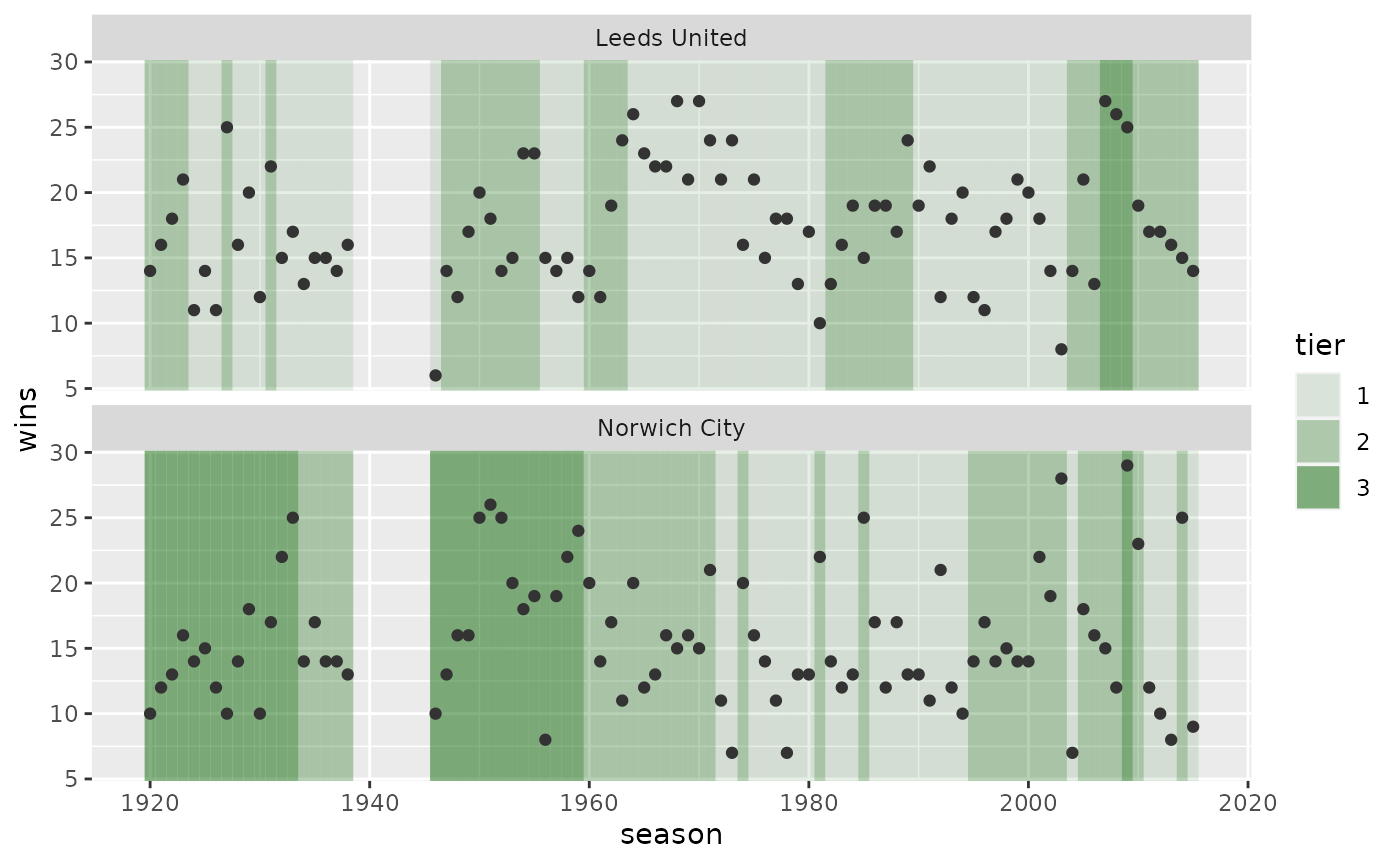
You can provide an argument, aes_y, where you can supply an expression just as you would for ggplot2:
uss_plot_seasons_tiers(leeds_norwich, aes_y = wins - losses)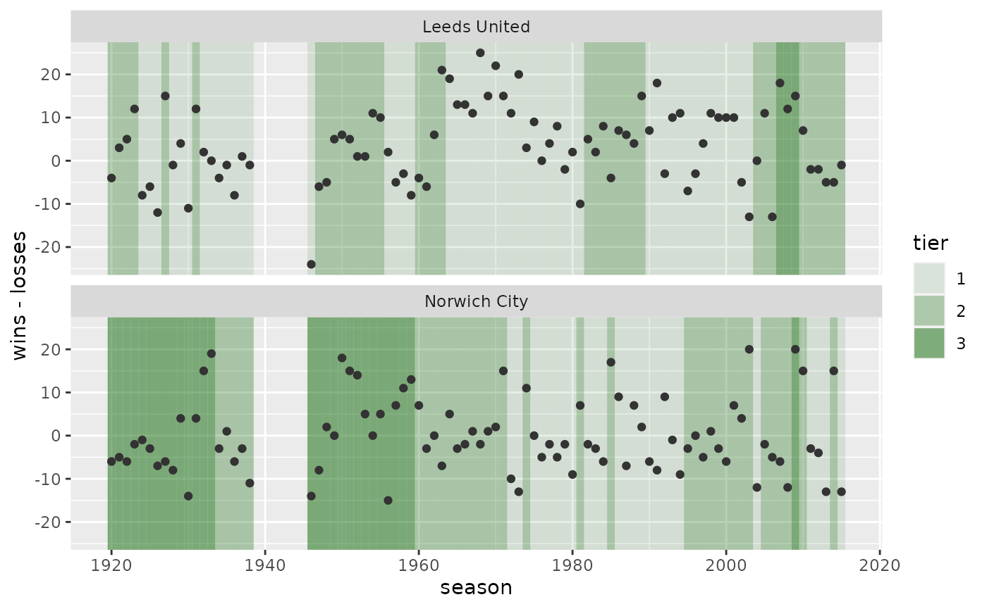
Add results
We use the vctrs package to help build a function, uss_result() that creates an S3 vector to display results:
uss_get_matches("italy") |>
  uss_make_teams_matches() |>
  mutate(
    result = uss_result(goals_for, goals_against),
    .after = opponent
  )
#> # A tibble: 50,808 × 10
#>    country tier  season team     date       at_home opponent    result goals_for
#>    <chr>   <fct>  <int> <chr>    <date>     <lgl>   <chr>       <uss_>     <int>
#>  1 Italy   1       1929 AC Milan 1929-10-06 TRUE    Brescia Ca…  W 4-1         4
#>  2 Italy   1       1929 AC Milan 1929-10-13 TRUE    Modena FC    W 1-0         1
#>  3 Italy   1       1929 AC Milan 1929-10-20 FALSE   SSC Napoli   L 1-2         1
#>  4 Italy   1       1929 AC Milan 1929-10-27 TRUE    AS Roma      W 3-1         3
#>  5 Italy   1       1929 AC Milan 1929-11-03 FALSE   Bologna FC   D 1-1         1
#>  6 Italy   1       1929 AC Milan 1929-11-10 TRUE    Inter        L 1-2         1
#>  7 Italy   1       1929 AC Milan 1929-11-17 FALSE   US Livorno   L 1-4         1
#>  8 Italy   1       1929 AC Milan 1929-11-24 TRUE    Lazio Roma   W 2-1         2
#>  9 Italy   1       1929 AC Milan 1929-12-08 FALSE   Juventus     L 1-3         1
#> 10 Italy   1       1929 AC Milan 1929-12-15 TRUE    US Cremone…  W 5-2         5
#> # … with 50,798 more rows, and 1 more variable: goals_against <int>
At this point, the only method defined for uss_result() is format(). The function is vectorised; the arguments must be the same length:
uss_result(c(1, 2, 3), c(2, 2, 2))
#> <ussie_result[3]>
#> [1] L 1-2 D 2-2 W 3-2